Categories: SummerBlogs
Professional Goals:
- Learn about medical device prototyping
- Develop computational simulation/modeling skills
- Understand how medical devices are optimized and manufactured
- Explore how physiology and pathophysiology can inform device design
Project: I will be conducting finite element analysis (FEA) on the DynaRing, a selectively compliant annuloplasty ring for mitral valve repair. I am exploring a forward problem, in which I am defining design parameters to simulate how the ring would deform in the heart. I am also interested in exploring the inverse problem, in which physiologic parameters can provide insights into design parameters, such as ideal material stiffnesses.
Week 1
Just getting started *virtually* in the lab. I have been installing and learning software tools like Solidworks and Abaqus. I have also been re-familiarizing myself with Onshape and finding some papers to guide my work. I have also been meeting with other members of the lab to frame my project and understand what I need to do. Ali referred me to a great resource (http://continuummechanics.org) to learn about concepts like tensors, stress, and strain, as well as some theory for FEA.
Week 2
I have been working on the forward problem. I learned how to create simple simulations on Solidworks. Then, I learned how to create assemblies by constructing the DynaRing in Solidworks. I also ran a linear, static study to simulate systole and diastole on the DyanRing. I had some difficulties with meshing because of poor contact definitions in the model. After resolving those, I used data from in vitro left heart simulator experiments with the DynaRing to define atrial and ventricular pressures acting on the DynaRing. See below for images from systole and diastole that show the displacement of the DynaRing (I applied maximum atrial and ventricular pressures during a cardiac cycle for now in the systole image; in the diastole image, I simply applied 11 kPa of pressure to the atrial surface, based on a quick Google search).
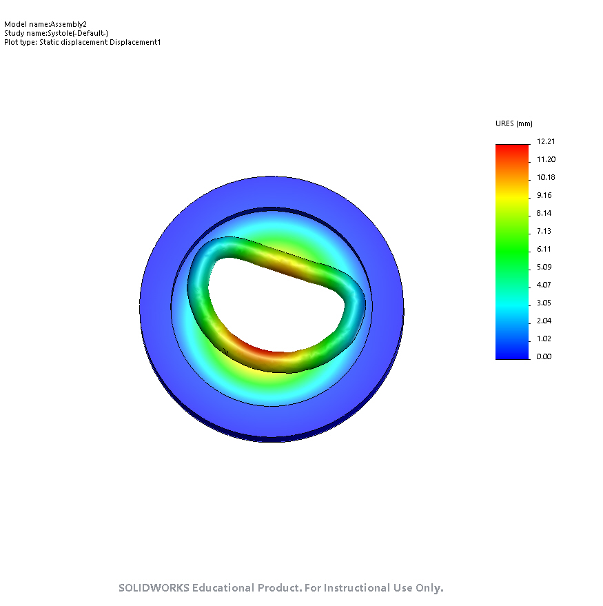
End-Systole
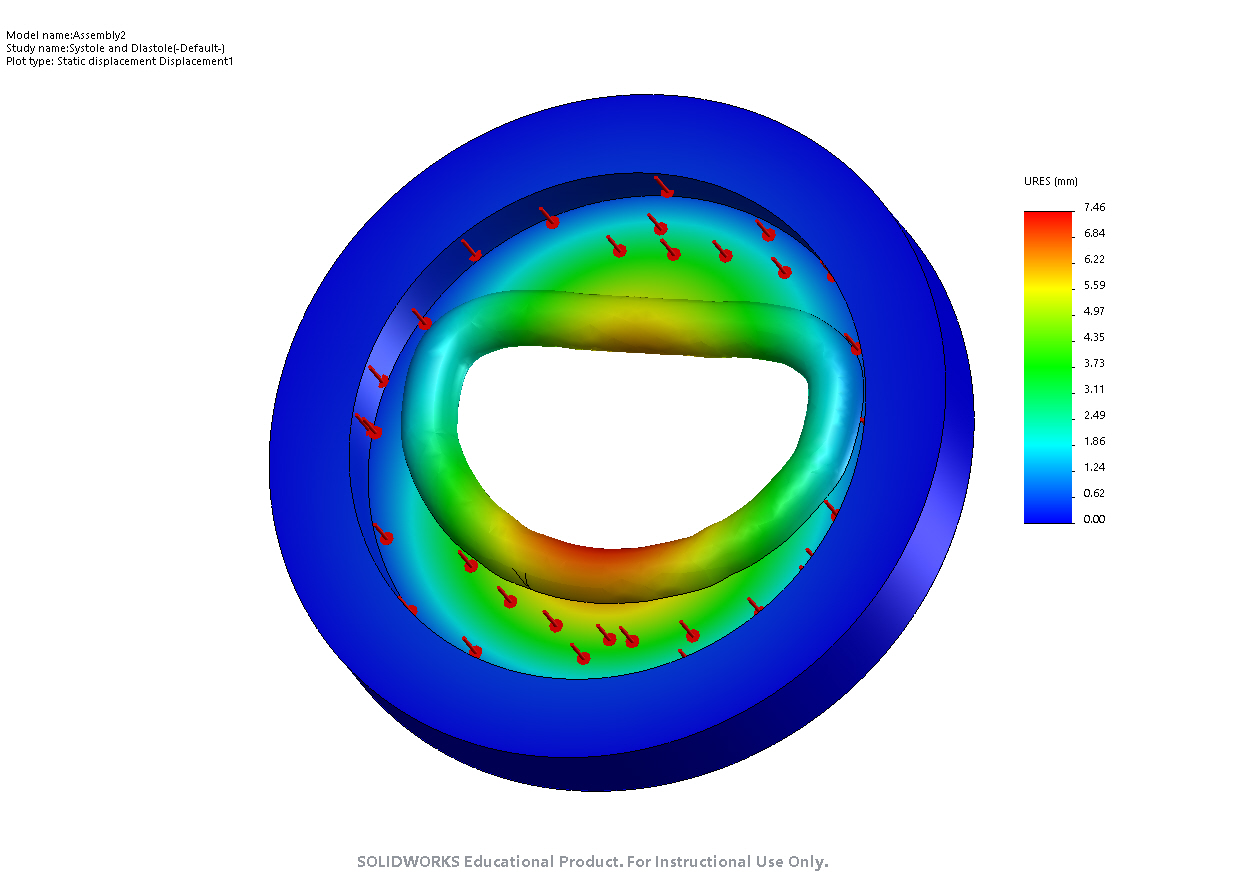
End-Diastole
My results are fairly consistent with the data presented in the conference paper written by Ali, Ileana, and Sam (for systole, I find a max displacement of 12.21mm and the paper reports 12.62mm max displacement). I still need to update my Young's modulus values for materials based on empirical data.
Week 3
I'm a bit more familiar with Solidworks now, but I still have a lot to learn. My main task currently is to extract important metrics from the DynaRing and observe how these metrics change during deformation in systole and diastole.
I defined several reference points at the core of the DynaRing based on anatomical landmarks. Specifically, I defined the anterior, posterior centers and the right and left commissures. See their reference locations on the image below.
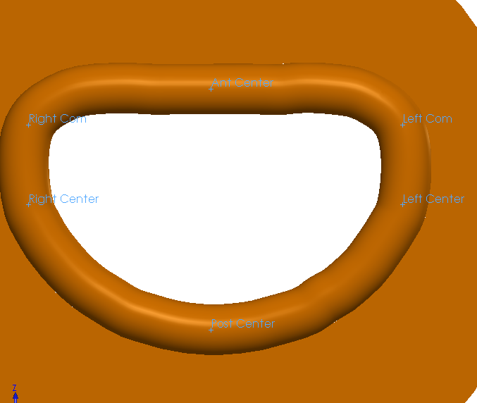
Reference Points
I defined sensors at these points to track how anterior-posterior diameter (AP diameter), intercommissural diameter (IC diameter), mitral orifice area (OA), and saddle height (SH), change over the course of systole or diastole.
I noticed that my calculated changes in these parameters at systole were dramatically smaller than the values reported in the conference paper figure (see below).
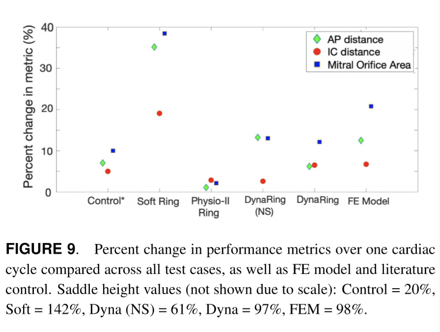
I considered evaluating how these metrics vary if instead of tracking changes at the reference points, I instead assumed the max changes possible based on the simulations I conducted (i.e. just apply the largest change possible irrespective of location). This appeared to be more consistent with the conference paper results. See the table below to observe the differences between the methodology of using reference points and using max changes.
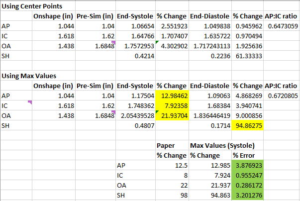
Initial Metrics Compared to Paper
Couple caveats: the orifice area (OA) was simply approximated as IC diameter x AP diameter for simplicity. I know this is not very accurate, but I just wanted a first-order approximation for now. I may update my methodology later, but it appears to be fine for now. Next, the IC diameter was evaluated with a slightly different method. I noticed that max changes in IC diameter occurred at nodes on the left and right ring segments that were nowhere near the commissures. So, I instead pulled out the maximum change in IC diameter from points close to the commissures. This was a lot more accurate for the comparison with the conference paper. If you are interested in replicating my results, I used Nodes 540941 and 544959 as references for IC diameter.
My next steps are to update Young's modulus values and start reading into using surrogate models to inform design.
Week 4
I met with Ali and received several important updates. 1) I now have empirical Young's modulus values based on the urethane + nitinol together 2) I realized that in my prior images, I was looking at resultant displacement rather than solely vertical displacement. My results were actually off. I also updated my sensors to not be the centers of each segment but rather the centers of the top surface of each segment (not interior of segments).
To fix my results, I updated Young's modulus values and also referenced Ali's prior solidworks simulations to apply pressure properly on the faces of the DyanRing. With proper adjustments, I was able to strongly replicate the results of the conference paper (OA is still estimated as a rectangular area).
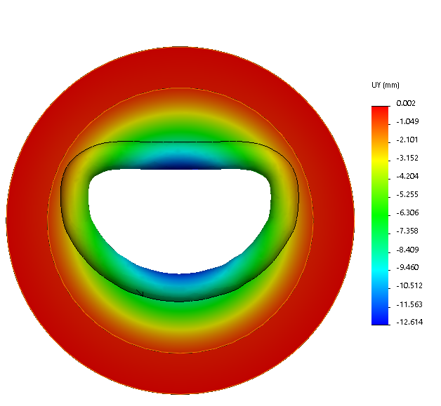
Vertical Displacement at End-Systole (Paper reports max of 12.62mm)
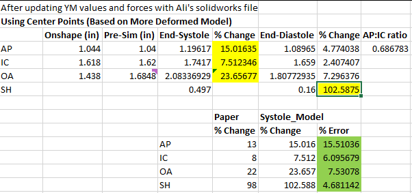
New Metrics Compared to Paper
One note is that AP diameter seems to be slightly off. I may need to update the pressures applied in systole and diastole to be more accurate. Second, I plan to update my orifice area calculation to be based on an integration of triangular areas between reference points on the DynaRing and the centroid of the ring. For now, a rectangular estimate appears to be fine.
My next task is to modify the Young's modulus values of the various segments and re-run these simulations. I want to determine how various metrics (AP, IC, SH) are affected by elasticity. I also need to find literature that describes ideal values for these metrics. After analyzing individual segments, I will look at pairs of segments and see how they change.
I also read Ali and Ileana's paper from their optimization course on using a surrogate model for design optimization. I am currently thinking of using a very similar process to describe the ideal material stiffness of the ring segments.
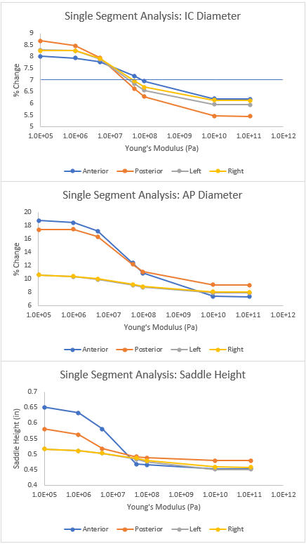
I performed single segment analysis of modulating Young's modulus (YM) to observe how a relevant metric (AP diameter for anterior/posterior segments and IC diameter for left/right segments) changes with variable stiffness. The maximum YM I tested was 110 GPa, which corresponds to titanium, which is about the hardest metail implant that would be considered for a mitral valve annuloplasty ring.
The results are below (plotting Young's modulus on log scale vs. % change on linear scale):
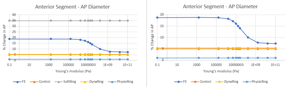
Anterior Segment Analysis (FE - Finite Element Model, DynaRing - Experimental Data on the Ring)
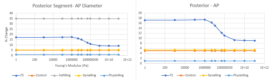
Posterior Segment Analysis
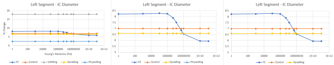
Left Segment Analysis
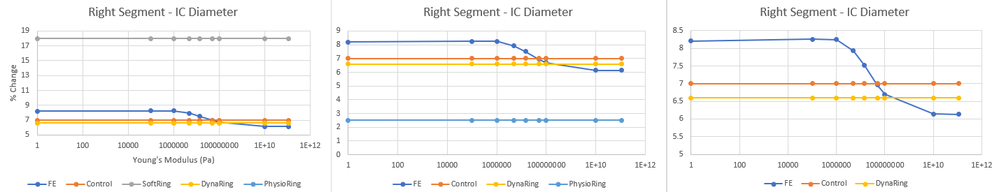
Right Segment Analysis
There were two important findings: 1. For the anterior and posterior segments, modifying each segment individually fails to achieve the desired % change in AP diameter associated with control. It appears we need to increase the stiffness of both the segments substantially to achieve this desired metric. However, I will say based on my results earlier in this blog, my model's % change in AP diameter was slightly higher than the value reported by the FE model in the conference paper, so my model may overestimate % change in AP diameter. Regardless, there needs to be substantial increase in YM values for the anterior and posterior segments.
2. For the left and right segments, it appears a YM of ~40 MPa and ~50MPa respectively, which are approximately 3-4x the current stiffness values, may be desired to achieve the control values reported in literature.
3. Again, this FE model may not be perfect and may need optimization. The general takeaways are that we may want to increase stiffnesses of each segment. Additionally, I may need to review my own model and ensure that a) my choice of sensors makes sense and b) my values for systole and diastole make sense.
Week 5
Towards the end of last week and the start of this week, my goal has been to conduct one at a time (OAT) sensitivity analysis. Essentially, I want to modify individual segments of the ring and observe how each metric is affected. Below are plots of my results:
Results of Sensitivity Analysis Comparing Changes in Metrics to Changes in Stiffness for Individual Segments
I also conducted ANOVA analysis and found that the AP diameter had a significant difference between segments. I then investigated which segments are significantly more sensitive to changes in elasticity in terms of affecting AP diameter. However, Ali pointed out how my data is nonlinear and not normally distributed, suggesting that we should explore other methods of statistical analysis.
With resources from Ali, I read about OAT sensitivity analysis. I found out that Spearman coefficients for correlation can be useful for nonlinear data that is monotonic, which applies to my data for this sensitivity analysis. If I had correlations for each segment, I could compare correlations between segments. However, I simply got a correlation coefficient of -1 for nearly all segments for every metric because my data was perfectly monotonic.
With initial insights from this sensitivity analysis, we decided to start looking into the optimization pipeline. We decided to use a surrogate model to optimize for AP, IC, and SH metrics. Currently my main two goals are 1) conduct proper sampling to build a surrogate model and 2) figure out what a good cost function would look like for our optimization.
Since I wanted to achieve good space-filling sampling to explore the full range of stiffnesses for each segment, I decided to use Latin Hypercube Sampling (LHS). I used the PyDOE package to implement this sampling and did some experimentation with different settings/criteria for the LHS. Ultimately, I found that using the 'maximin' criterion resulted in the largest degree of space filling.
I discretized my sample space into 10 bins: each sample consists of 4 stiffness values ranging between 1e5 to 1.1e11 Pa in stiffness. I then used the FE model I built on Solidworks to run simulations given these stiffness conditions at systole and diastole (total 20 simulations). Then, for each simulation, I extracted % change in AP diameter, % change in IC distance, and saddle height. I now have my training data set for a surrogate model.
My next step is to read into cost functions and continue refining my optimization pipeline.
Week 6
My goal for this week is to start carrying out my optimization pipeline detailed below:
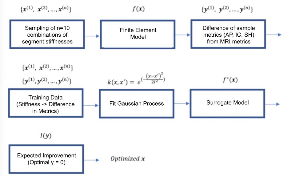
Optimization Overview
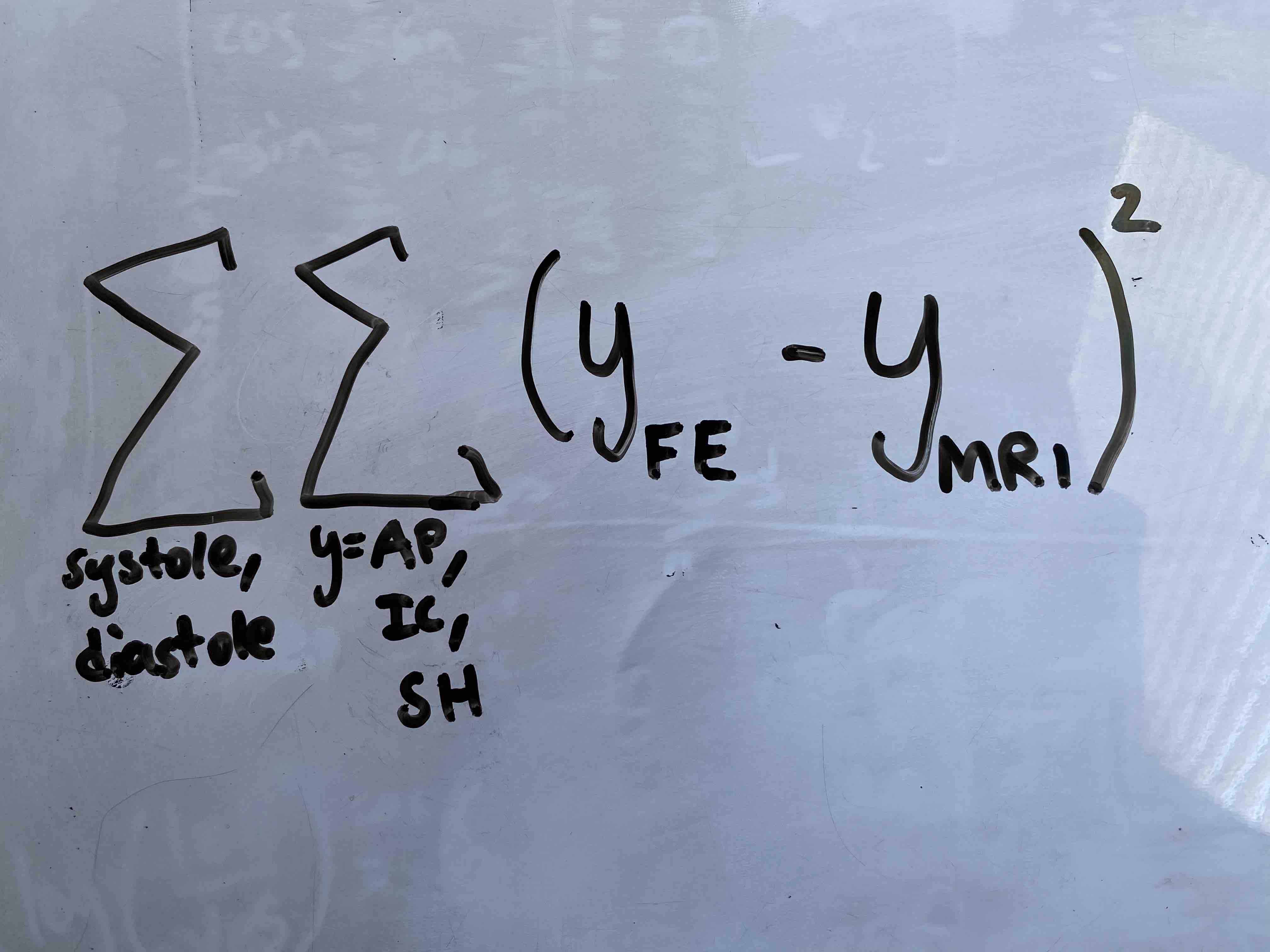
1. Build a training data set: I used LHS to obtain 10 samples as detailed above in Week 5. In brief, each sample consists of 4 stiffness values for each segment of the ring. I then simulated systole and diastole on my FE model to construct a training data set, with the outputs being AP, IC, and SH. Specifically, I will be defining my output as a scalar that is the sum at two time points of the square of the difference between FE model metrics and MRI metrics:
2. Apply Gaussian Process (GP) to build surrogate model: I plan to use scikit-learn to develop the surrogate model.
3. Use Expected Improvement (EI) Acquisition to find stiffness combinations that minimize the surrogate model.
07/25/20 So far, I have successfully built a training data set and implemented a basic gaussian process script. I need to refine my cost function and further generalize my current code for the Gaussian process to incorporate higher-dimensional data, as I have 5 total dimensions to evaluate in my optimization pipeline (4 stiffness values, 1 cost function value).
I used Martin Krasser's blog as a reference: http://krasserm.github.io/2018/03/19/gaussian-processes/?fbclid=IwAR098o-wkA8SovHSui1LAL8iPrCLiCSxOIqEd79JFGvL5votzhSwtZktLO4.
Week 7
This week has been focused on optimization. My goal by the end of the summer is to incorporate MRI data into my optimization pipeline and understand patient-specific variations in ideal ring stiffnesses.
One main thing I did this week was find literature confirming that expected improvement was the best Bayesian optimization algorithm for our project. I also found literature suggesting that mitral orifice area may be a redundant parameter and not necessary. Last, Ali, Ileana, and I discussed how to properly define saddle height, and we are currently evaluating it as a ratio with IC distance (SH:IC ratio, expressed as %).
Another major thing I did this week was learn about Bayesian optimization and implement an expected improvement algorithm, using Martin Krasser's Blog (http://krasserm.github.io/2018/03/21/bayesian-optimization/). I had a lot of trouble with converting the 1-dimensional algorithm provided by the blog into a multidimensional one, but I finally modified the code in order to achieve this.
One important thing I will do now is confirm the effectiveness of this optimization pipeline by creating a mock dataset that should result in a certain combination of stiffnesses that I know are ideal. This can help me debug the code that I have currently.
Next week, I will be gearing up to actually implement this optimization pipeline, after discussing with Ali and Ileana that our pipeline is accurate and ready to deploy.
Week 8
I started executing my optimization pipeline fully this week! Specifically, as an initial control, I created a heatmap of cost function across stiffnesses of the anterior/posterior segments. As a reminder, I found that these two segments were qualitatively the most influential on our mitral valve metrics in my prior sensitivity analysis. See the heat map below:
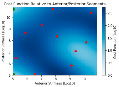
Red dots represent initial sample points and green dots (in upper left and bottom left corners) represent each successive design point selected by optimization
As seen in the heatmap, the optimization algorithm appears to be initially working because the predicted next points, shown in green, are indeed in regions of low cost function. This initial result is promising.
On Thursday, I ran 20 simulations of stiffness combinations predicted as optimal by the optimization pipeline. There must be an error, because I could not achieve convergence. Some of my samples did achieve a low cost function (minimum of ~9), but the expected improvement exploration algorithm failed to converge at any particular point. I am not sure why this is happening. Some ideas I had include the fact that the design space is enormous. I may want to have a larger training dataset using LHS.
I also tried to play around with the zeta hyperparameter in the expected improvement algorithm, which defines how much exploration to allow in optimization. I set this to extremely low values, indicating minimal exploration in the hopes of achieving a convergence, but this did not happen.
Next week, I need to figure out why this is not working, and I need to start extracting patient-specific metrics from MRI data.
Week 9
I started this week by re-evaluating how I am defining my mitral valve metrics with Ali and Ileana. Specifically, I had some initial MATLAB code to plot changes in mitral valve points throughout the cardiac cycle from Sam. My goal was to extract patient-specific mitral valve metrics.
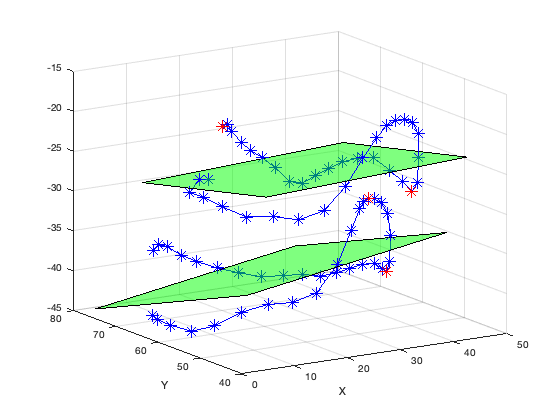
Ileana found a paper (https://www.ahajournals.org/doi/full/10.1161/CIRCULATIONAHA.104.525485), which defined a least squares plane for mitral valve points to evaluate saddle height. I used this paper's definition to recalculate saddle height for 7 patient samples from a control group (healthy hearts). The below figure shows a sample from one patient, with mitral valve geometry at systole and diastole plotted (systole is above diastole), and each segment of the mitral valve colored. The least squares plane is also shown in yellow.
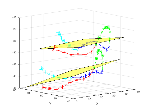
Illustration of MRI segmentation and least-squares plane fitting at systole (top) and diastole (bot). Red = right, green = posterior, blue = left, cyan = anterior
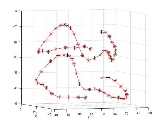
Calculation of Saddle Height. Two points (shown in red) with the largest positive and negative orthogonal displacements from plane were used.
While on this topic, I also reconsidered how to properly calculate IC distance and AP diameter. IC distance was defined as the largest distance between the left and right segments of the mitral annulus. For AP diameter, I defined two major approaches that are shown in the images below. First, the peak-to-peak method involved finding the two largest peaks, one on anterior and one on posterior segment of the mitral annulus, and finding the Euclidean distance between the two points. The second method involved projecting all mitral annulus points orthogonally onto the least squares plane. I then evaluated the largest distance between the anterior and posterior segments of the mitral annulus.
Peak-to-Peak Method for AP Diameter Calculation. Blue points indicate the reference points used to calculate AP diameter.
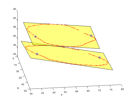
Orthogonal Projection Method for AP Diameter Calculation. Blue points indicate the reference points used to calculate AP diameter.
The below table highlights how the AP diameter is different between the two methods. I need to determine which method is better to proceed with.
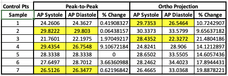
AP Diameter Comparison Between Two Methods. Highlighted cells indicate that AP was larger at systole than diastole.
I have finalized my methods for obtaining metrics from MRI data. 1) For saddle height, I am continuing my method from above, in which I sum the orthogonal distances between the highest and lowest points. 2) For AP diameter, I am picking two markers (indices 14, 32) and calculating the distance between the two orthogonal projections of these points on a plane. See the figure above for an example of these orthogonal projections. 3) For IC distance, I am following the exact same method as AP diameter, using markers at indices 5 and 23 as my two reference points to evaluate IC distance. 4) I am still debating the best way to calculate orifice area. Currently, I am taking the convexhull() function of the raw, 3D data
Beyond calculating these patient metrics, I also debugged my optimization code using expected improvement exploration. I was able to attain convergence using literature values as a set, optimal point. The minimum cost function I achieved was ~14.