- NewStrainGageCalibration

- TestTrackStrainGageTest

RiSE Leg Strain Gage Test and Calibration

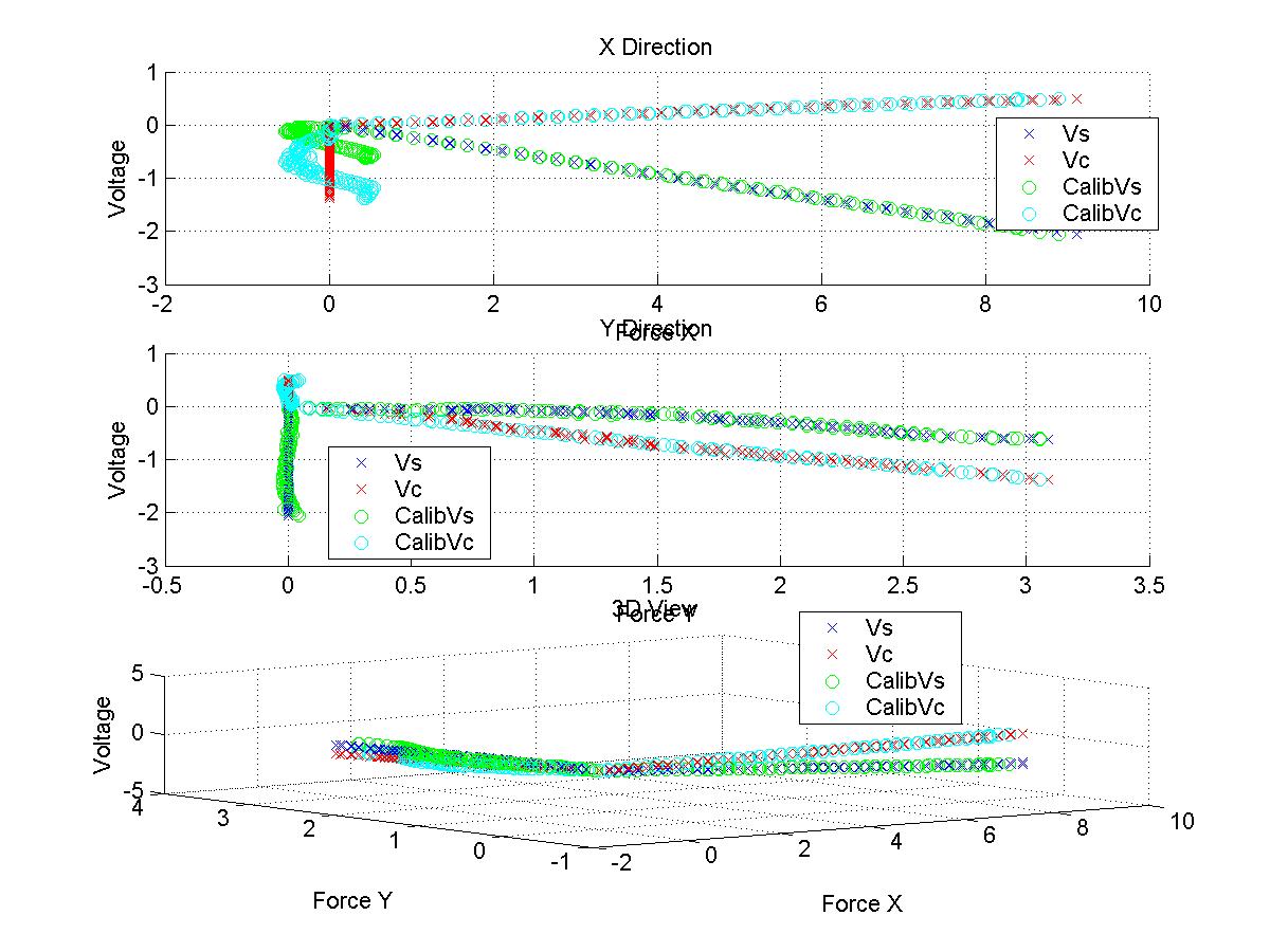
-- JonathanKarpick - 08 Sep 2004:

• Re-did pseudo Inverse with all data at the same time, taking the initial zero reading as the offset and then doing C=F*pinv(V) (same as C=F/V):
  C = [-3.9742, 1.4454; -0.4903 -1.9995]
  for C=[Cxs Cxc; Cys Cyc]
• YongLae's test data:
  
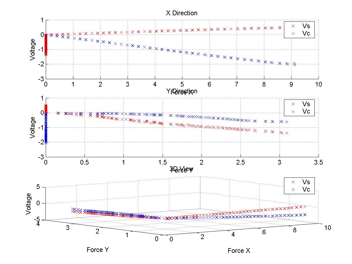
• Test data with subsequent fit:
  
• MATLAB Script attached:
  StrainGageTestData.m

-- YongLaePark - 30 Aug 2004

Objective

• Read the forces RiSE legs take through strain gages while climbing and give them as inputs to control the robot for better climbing

Test Setup and Measurement

• Strain gages are attached on both sides of each spring which connects the lower leg and the upper leg as shown in the picture.
• Constant increase of in one directional (either x or y axis) displacement has been made on the leg using a height gage.
• On each displacement, applied force and output voltages (V_s and V_c) from strain gages are measured using a scale and multimeters.
  • V_s: Voltage output from spring s (straight).
  • V_c: Voltage output from spring c (curved).

Test 1: Displacement in x axis

• Displacement of the the feet has been made only in x axis, and the applied force and voltage outputs are measured.

• Displacement was made up to 0.4 inch in every 0.01 inch.

• Test setup:
  

• Test Result:
  

• Test Data: StrainGageTestData_X.xls

Test 2: Displacement in y axis

• Displacement of the the feet has been made only in y axis, and the applied force and voltage outputs are measured.

• Displacement was made up to 0.5 inch in every 0.01 inch.

• Test setup:
  

• Test Result:
  

• Test Data: StrainGageTestData_Y.xls

Calibration

Calibration Matrix (C)

1. Pseudo Inverse

• Since we are interested in how the voltage change affect the force change (not the intercept of the F-V graph but the coefficients), I moved all the measured V_s and V_c data in parallel where the initial points (when the force is 0) meet zero. Then, I performed the same pseudo inverse.

• F = C * V => C = F * pinv(V)
  • F: 2 x n force matrix
  • V: 2 x n output voltage matrix
  • C: 2 x 2 calibration matrix

      F_x = |f_x1, f_x2, ..., f_xn|      F_y = |  0 ,   0 , ...,   0 |  
            |  0 ,   0 , ...,   0 |            |f_y1, f_y2, ..., f_yn|
      V_1 = |v1_s1, v1_s2, ..., v1_sn|   V_2 = |v2_s1, v2_s2, ..., v2_sn|
            |v1_c1, v1_c2, ..., v1_cn|         |v2_c1, v2_c2, ..., v2_cn|
      C = |c11, c12|
          |c21, c22|

      C_x = F_x * pinv(V_1)
      C_y = F_y * pinv(V_2)

• Result
  • C_x = [ -6.7593, -9.9989 ; 0, 0 ] - Calibration matrix with x-axis force (Test 1)
  • C_y = [ 0, 0 ; -0.4243, -1.9885 ] - Calibration matrix with y-axis force (Test 2)
  • Therefore, calibration matrix is: C = [ -6.7593, -9.9989 ; -0.4243, -1.9885 ]

2. Pseudo Inverse at the same time

• F = C * V

      |F_x,  0 | = |c11, c12| * |V_1, V_2|
      | 0 , F_y|   |c21, c22|  

• Result
  • C = [ -3.9665, 1.3981 ; -0.4790, -1.9691 ]

3. One Variable Pseudo Inverse

• I calculated only c11 and c22 assuming c12 and c21 are zero (ignoring V_c in Test 1 and V_s in Test 2) using pseudo inverse. In this case, the measured data were moved in parallel to have zero initial points.

• Result
  • C = [ -4.3258, 0 ; 0, -2.1372 ]

4. Simple Linear Regression

• Since it is clear that V_s is more important for Test 1(x-axis force) and V_c for Test 2(y-axis force), I performed simple linear regression to find the best fit slopes, s1 and s2, of F-V_s plot in Test 1 and F-V_c plot in Test 2, which are comparable with c11 and c22 in matrix C.

• Result
  • Test 1: F = - 4.3604 * V_s + 9.1307 => s1 = -4.3604
  • Test 2: F = - 2.1510 * V_c + 4.4151 => s2 = -2.1510
  • C = [ -4.3604, 0 ; 0, -2.1510 ]

Result Comparison

• F vs V_s (Test 1):
  

• F vs V_c (Test 2):