new web: http://bdml.stanford.edu/pmwiki
TWiki > Main Web>PerchingProject>ElenaStanfordPage (07 Jan 2011, ElenaGlassman)
Elena's Perching Page while at Stanford:
If a trajectory ended in the ROA of an existing trajectory, but not on the trajectory, then the ROA for the endpoint of that new trajectory would be smaller (I'm pretty sure) than if it had ended on the existing trajectory, since the ROA of the endpoint of the new trajectory has to fall entirely within the ROA of the trajectory it's feeding in to.
Also, if an optimizer like SNOPT has found a trajectory endpoint in the ROA of an existing trajectory, how much "harder" could it be to add some time to the new trajectory and actually connect it to the existing trajectory?
Note: the ultimate connection point may be at a point "far downstream" of the trajectory waypoint whose associated ROA the endpoint initially fell in to. I guess, to be technically correct, I should say funnel time-slice, rather than ROA of a trajectory waypoint, because the latter terminology suggests that points in that waypoint "ROA" will go to that waypoint, rather than thinking of the ROA as the slice of a funnel in which all trajectories approach the associated nominal trajectory.
The fact that we're considering purely passive trajectories [we are not steering the plane toward existing trajectories] suggests that trajectories that connect back to the tree would all connect at the static equilibrium (root tree node).
So, it looks like we have two choices in terms of tree structure, depending on whether or not we force new trajectories to connect back to tree or just let them end somewhere in the funnel of an existing trajectory (perhaps with a preference for a location nearer, rather than farther, to the center of that funnel): if we choose the former option, we might get a spaghetti-like structure all coming out of the static equilibrium, and if we choose the latter option, we might get more of a tree-like structure, with branches coming off of branches, but with possibly thinner funnels. Remaining progress to report on:
Also, we need at least second order terms for the Taylor expansion of the dynamics, because the friction model is of just Coulomb friction, and the high slope of the Coulomb friction approximation at the linearization point is going to adversely affect the accuracy of the Taylor approximation a LOT unless there are higher order terms to capture its plateaus. We could leave out the friction term, but then the resulting ROA would be for the frictionless model; there's no control on which to tag a feedforward model of the friction--oh wait!! What if our "passive controller" for the TI ROA calculation was just the forces from the friction model? Would that make sense? I'm not sure which is better/more accurate: calculating a high order Taylor expansion of the dynamics and calculating the TI ROA with no input or calculating a less high order Taylor expansion of the frictionless dynamics and calculating the TI ROA for a controller which is actually just imposing the forces from the friciton model.
Since Alexis can generate the same symbolic gradients I'm trying to generate with the generate_dynamics_func_gradients (but doesn't package them like our code does), and I am not getting traction on what is most likely a memory issue with our code, I think we'll have to write a script to use Alexis' MotionGenesis? to generate the first, second, and perhaps third order terms of the Taylor series, which will of course be high-dimensional tensors.
 And my last attempt at finding the Jacobian turns out to have given me a matrix of NaN? . We'll have our more powerful version of MotionGenesis? up and running soon, so this seems like an appropriate time to put my classwork-hat back on.
[2,3]Dec2010 Not Just Describing the Symptoms, but Understanding the Underlying Phenomena
Suddenly, memory (virtual, physical, swap files, etc.) management has become very interesting! I've found the following pages helpful: [not an exhaustive list]
And my last attempt at finding the Jacobian turns out to have given me a matrix of NaN? . We'll have our more powerful version of MotionGenesis? up and running soon, so this seems like an appropriate time to put my classwork-hat back on.
[2,3]Dec2010 Not Just Describing the Symptoms, but Understanding the Underlying Phenomena
Suddenly, memory (virtual, physical, swap files, etc.) management has become very interesting! I've found the following pages helpful: [not an exhaustive list] 
The input arguments of the "lyap" command must be numeric arrays. I was just feeding it the symbolic A! Silly me. Will evaluate A at the equilibrium point, with all the model parameter values substituted in. I can do this one of two ways: (1) work on the auto-generated gradients .m file, since that can be used to spit A out with everything substituted in or (2) sub things in myself using subs commands, etc. I prefer option 1, since that's how it'll be done in the robotlib code. However, Matlab won't let me use its editor, because the file's too big, and XCode, which I was using before, just crashed. Aquamacs was recommended online for working with large text files on a Mac. Installing it now. Opens it up; doesn't freeze up. Way to go, Aquamacs, you're the... program? :-P By the way, Aquamacs installation: drag icon to the Applications folder. Done. Traditional GNU Emacs installation? Run configure. Browse error messages. Apend commands to configure command and re-run. Then make. Then make install. Then... it refuses to open. Why the long, drawn-out (failed) install process when another program can do it so cleanly? Grr. Now I need to evaluate the Jacobian at the static equilibrium point, right? Yes. The equilibrium point of the linearized dynamics or the nonlinear dynamics? Shouldn't those two points be the same, if the system is started from an initial condition close enough to the goal? The friction terms have been removed; what does that mean for this particular hybrid state? The friction term(s) Alexis left out of the hybrid state I'm working on right now are not "active" at the static equilibrium because it's just the friction between the tail and the wall and is zero when the system is at rest. Fixed the script that produces the .m file of gradients based on the symbolic derivatives (which saves us the time consuming step of using slow symbolic toolbox functions like subs, etc.) and talked to Alexis. The rest point Alexis found by numerical simulation: x y qa qH qK qS x' y' qa' qH' qK' qS'
(m) (m) (deg) (deg) (deg) (m) (m/s) (m/s) (deg/s) (deg/s) (deg/s) (m/s) -1.077673E-01 -9.706154E-02 9.434811E+01 1.069099E+02 9.138784E+01 1.145137E-03 -2.475994E-08 5.670911E-09 1.213560E-06 5.527654E-06 -2.378733E-06 4.361853E-09 Packaging that up in to the state vector: [qA; qH; qK; qS; x; y; qAp; xp; yp] = [9.434811E+01; 1.069099E+02; 9.138784E+01; 1.145137E-03; -1.077673E-01; -9.706154E-02; 1.213560E-06; -2.475994E-08; 5.670911E-09] I'll plug that into the dynamics function that computes the state derivative for given state, and confirm that this is indeed a static equilibrium for the model I packaged into a robotlib plant object. Whoops! The code used to find the Jacobian has a different ordering of the variables than in the robotlib plant object. I'll multiply A by a row-switching matrix, then a column switching matrix, to make it match the robotlib plant. Is that easier than changing the robotlib plant? Nope. Changing plant now. Order consistent with Alexis' Jacobian:
If a trajectory ended in the ROA of an existing trajectory, but not on the trajectory, then the ROA for the endpoint of that new trajectory would be smaller (I'm pretty sure) than if it had ended on the existing trajectory, since the ROA of the endpoint of the new trajectory has to fall entirely within the ROA of the trajectory it's feeding in to.
Also, if an optimizer like SNOPT has found a trajectory endpoint in the ROA of an existing trajectory, how much "harder" could it be to add some time to the new trajectory and actually connect it to the existing trajectory?
Note: the ultimate connection point may be at a point "far downstream" of the trajectory waypoint whose associated ROA the endpoint initially fell in to. I guess, to be technically correct, I should say funnel time-slice, rather than ROA of a trajectory waypoint, because the latter terminology suggests that points in that waypoint "ROA" will go to that waypoint, rather than thinking of the ROA as the slice of a funnel in which all trajectories approach the associated nominal trajectory.
The fact that we're considering purely passive trajectories [we are not steering the plane toward existing trajectories] suggests that trajectories that connect back to the tree would all connect at the static equilibrium (root tree node).
So, it looks like we have two choices in terms of tree structure, depending on whether or not we force new trajectories to connect back to tree or just let them end somewhere in the funnel of an existing trajectory (perhaps with a preference for a location nearer, rather than farther, to the center of that funnel): if we choose the former option, we might get a spaghetti-like structure all coming out of the static equilibrium, and if we choose the latter option, we might get more of a tree-like structure, with branches coming off of branches, but with possibly thinner funnels. Remaining progress to report on:
Also, we need at least second order terms for the Taylor expansion of the dynamics, because the friction model is of just Coulomb friction, and the high slope of the Coulomb friction approximation at the linearization point is going to adversely affect the accuracy of the Taylor approximation a LOT unless there are higher order terms to capture its plateaus. We could leave out the friction term, but then the resulting ROA would be for the frictionless model; there's no control on which to tag a feedforward model of the friction--oh wait!! What if our "passive controller" for the TI ROA calculation was just the forces from the friction model? Would that make sense? I'm not sure which is better/more accurate: calculating a high order Taylor expansion of the dynamics and calculating the TI ROA with no input or calculating a less high order Taylor expansion of the frictionless dynamics and calculating the TI ROA for a controller which is actually just imposing the forces from the friciton model.
Since Alexis can generate the same symbolic gradients I'm trying to generate with the generate_dynamics_func_gradients (but doesn't package them like our code does), and I am not getting traction on what is most likely a memory issue with our code, I think we'll have to write a script to use Alexis' MotionGenesis? to generate the first, second, and perhaps third order terms of the Taylor series, which will of course be high-dimensional tensors.
And my last attempt at finding the Jacobian turns out to have given me a matrix of NaN? . We'll have our more powerful version of MotionGenesis? up and running soon, so this seems like an appropriate time to put my classwork-hat back on.
[2,3]Dec2010 Not Just Describing the Symptoms, but Understanding the Underlying Phenomena
Suddenly, memory (virtual, physical, swap files, etc.) management has become very interesting! I've found the following pages helpful: [not an exhaustive list]
The input arguments of the "lyap" command must be numeric arrays. I was just feeding it the symbolic A! Silly me. Will evaluate A at the equilibrium point, with all the model parameter values substituted in. I can do this one of two ways: (1) work on the auto-generated gradients .m file, since that can be used to spit A out with everything substituted in or (2) sub things in myself using subs commands, etc. I prefer option 1, since that's how it'll be done in the robotlib code. However, Matlab won't let me use its editor, because the file's too big, and XCode, which I was using before, just crashed. Aquamacs was recommended online for working with large text files on a Mac. Installing it now. Opens it up; doesn't freeze up. Way to go, Aquamacs, you're the... program? :-P By the way, Aquamacs installation: drag icon to the Applications folder. Done. Traditional GNU Emacs installation? Run configure. Browse error messages. Apend commands to configure command and re-run. Then make. Then make install. Then... it refuses to open. Why the long, drawn-out (failed) install process when another program can do it so cleanly? Grr. Now I need to evaluate the Jacobian at the static equilibrium point, right? Yes. The equilibrium point of the linearized dynamics or the nonlinear dynamics? Shouldn't those two points be the same, if the system is started from an initial condition close enough to the goal? The friction terms have been removed; what does that mean for this particular hybrid state? The friction term(s) Alexis left out of the hybrid state I'm working on right now are not "active" at the static equilibrium because it's just the friction between the tail and the wall and is zero when the system is at rest. Fixed the script that produces the .m file of gradients based on the symbolic derivatives (which saves us the time consuming step of using slow symbolic toolbox functions like subs, etc.) and talked to Alexis. The rest point Alexis found by numerical simulation: x y qa qH qK qS x' y' qa' qH' qK' qS'
(m) (m) (deg) (deg) (deg) (m) (m/s) (m/s) (deg/s) (deg/s) (deg/s) (m/s) -1.077673E-01 -9.706154E-02 9.434811E+01 1.069099E+02 9.138784E+01 1.145137E-03 -2.475994E-08 5.670911E-09 1.213560E-06 5.527654E-06 -2.378733E-06 4.361853E-09 Packaging that up in to the state vector: [qA; qH; qK; qS; x; y; qAp; xp; yp] = [9.434811E+01; 1.069099E+02; 9.138784E+01; 1.145137E-03; -1.077673E-01; -9.706154E-02; 1.213560E-06; -2.475994E-08; 5.670911E-09] I'll plug that into the dynamics function that computes the state derivative for given state, and confirm that this is indeed a static equilibrium for the model I packaged into a robotlib plant object. Whoops! The code used to find the Jacobian has a different ordering of the variables than in the robotlib plant object. I'll multiply A by a row-switching matrix, then a column switching matrix, to make it match the robotlib plant. Is that easier than changing the robotlib plant? Nope. Changing plant now. Order consistent with Alexis' Jacobian: Finally!
Back to evaluating our corrected Jacobian at this verified equilibrium point and solving for a quadratic Lyapunov candidate using the following command in Matlab: S = lyap(Jacobian',eye(n)), where n is the number of states.
9Dec2010 Everything that could go wrong, has gone wrong. :-P
Note to self: if you set gamma to anything, even [], before running any code that refers to the gamma variable in Alexis' dynamics/derivatives, Matlab won't think of the gamma function and refuse to run your code.
 There is no B matrix, just the A matrix, the way this is being called, so I guess, in this case, since A has one extremely small eigenvalue that is effectively zero (5.713486169742567e-13), the lyap command will not work. Hmmm... This step was just for computing a Lyapunov candidate (I'm guessing as a starting point for the region of attraction code). I'm very interested to know whether the solution is nonexistant or not unique. If it's not unique, all I want is one! What if I added just enough "noise" to the Jacobian to put it over the threshold in terms of rank, then got that noisy matrix's lyapunov candidate. It's just a starting point...
Emailing Mark T and Russ to discuss.
Okay, heard back from Mark T, did some more follow-up analysis, and talked to Alexis. Will sleep on all that, and reflect/write tomorrow.
10Dec2010 Breakthrough!!
Before I summarize Alexis, Mark T, Russ, and my discussion last night, I need to say that we finally have a breakthrough. I corrected a silly mistake and decided I will never (if possible) create systems that represent their states in different units than the units used internally for calculations because it's just asking for trouble. More importantly, I determined that y is in fact defined in such a way that the system dynamics are invariant to its value. That is why the Jacobian was not full rank. I removed the y variable from the state, leaving y', it's derivative, which does affect other variables. Alexis thought absolute y should affect other variables, but MotionGenesis? says otherwise. He was drawing diagrams where y was the vertical position of the center of gravity of the plane, which is between two wall attachment points (the spines and tail), saying that if y changes, all the other variables should change. This makes sense to me, but it makes equal sense to me that y could be defined differently so that the system is invariant to absolute y.
Anway, I removed y from the state since it's not in the EOM and now we have a candidate lyapunov function for the passive, stuck-on-the-wall, frictionless system, which for which I'm about to attempt calculating a region of attraction!
13Dec2010 More Interesting Conceptual Discussions, Plus: a Region of Attraction Might Be Closer than I Had Thought Yesterday!
Quick update:
There is no B matrix, just the A matrix, the way this is being called, so I guess, in this case, since A has one extremely small eigenvalue that is effectively zero (5.713486169742567e-13), the lyap command will not work. Hmmm... This step was just for computing a Lyapunov candidate (I'm guessing as a starting point for the region of attraction code). I'm very interested to know whether the solution is nonexistant or not unique. If it's not unique, all I want is one! What if I added just enough "noise" to the Jacobian to put it over the threshold in terms of rank, then got that noisy matrix's lyapunov candidate. It's just a starting point...
Emailing Mark T and Russ to discuss.
Okay, heard back from Mark T, did some more follow-up analysis, and talked to Alexis. Will sleep on all that, and reflect/write tomorrow.
10Dec2010 Breakthrough!!
Before I summarize Alexis, Mark T, Russ, and my discussion last night, I need to say that we finally have a breakthrough. I corrected a silly mistake and decided I will never (if possible) create systems that represent their states in different units than the units used internally for calculations because it's just asking for trouble. More importantly, I determined that y is in fact defined in such a way that the system dynamics are invariant to its value. That is why the Jacobian was not full rank. I removed the y variable from the state, leaving y', it's derivative, which does affect other variables. Alexis thought absolute y should affect other variables, but MotionGenesis? says otherwise. He was drawing diagrams where y was the vertical position of the center of gravity of the plane, which is between two wall attachment points (the spines and tail), saying that if y changes, all the other variables should change. This makes sense to me, but it makes equal sense to me that y could be defined differently so that the system is invariant to absolute y.
Anway, I removed y from the state since it's not in the EOM and now we have a candidate lyapunov function for the passive, stuck-on-the-wall, frictionless system, which for which I'm about to attempt calculating a region of attraction!
13Dec2010 More Interesting Conceptual Discussions, Plus: a Region of Attraction Might Be Closer than I Had Thought Yesterday!
Quick update:  that is found experimentally, via sampling, to contain dynamics for which the time derivative of the lyapunov candidate is less than or equal to zero (see below).
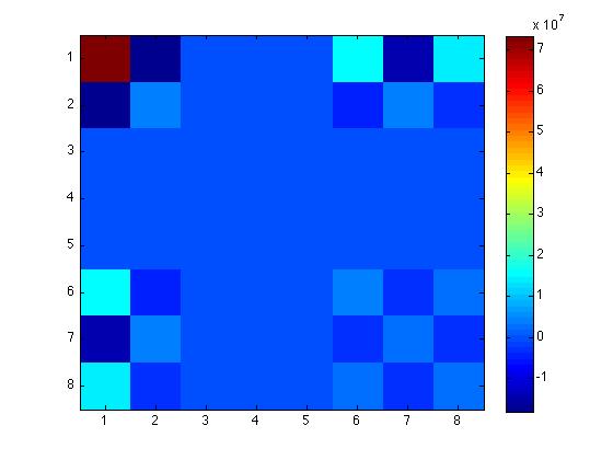 If the elements along the diagonal were largest, then level sets of the Lyapunov function would correspond to roughly "ball-like" ROAs in the appropriately scalled 8 dimensional state space. But in this case, we have one very large diagonal element (corresponding to x, the horizontal position of the COM) and next largest are at the 1,6 and 1,8 position in the matrix. What does that mean? Well, if we're visualizing the relative steepness of this lyapunov function over various axes, then this function is incredibly steep when moving along the x axis away from the equilibrium point. Does that make sense? Given that the tail is attached to the wall by a very stiff spring in this hybrid state, x probably has a large effect on things. And that spring is exerting restoring forces, so wouldn't a good lyapunov function candidate be such that, for a given rho, the levelset (ROA) is "wide" along the x axis? That's the opposite of what we have here from the lyapunov candidate produced by the Matlab lyap command as a function of the linearized dynamics. How much of the restoring spring's effects on the system dynamics are captured in the linearized dynamics? It's typically modeled as force = -kx, so that's certainly captured in the linearization, and so the lyapunov candidate is different than what I'd expect.
Let's look at the linearized dynamics, which is all the lyap command knows. Uh oh, they're nothing like what I expected. (Then again, what was I expecting?)
So, apparently, the Jacobian, when evaluated at the static equilibrium, is:
If the elements along the diagonal were largest, then level sets of the Lyapunov function would correspond to roughly "ball-like" ROAs in the appropriately scalled 8 dimensional state space. But in this case, we have one very large diagonal element (corresponding to x, the horizontal position of the COM) and next largest are at the 1,6 and 1,8 position in the matrix. What does that mean? Well, if we're visualizing the relative steepness of this lyapunov function over various axes, then this function is incredibly steep when moving along the x axis away from the equilibrium point. Does that make sense? Given that the tail is attached to the wall by a very stiff spring in this hybrid state, x probably has a large effect on things. And that spring is exerting restoring forces, so wouldn't a good lyapunov function candidate be such that, for a given rho, the levelset (ROA) is "wide" along the x axis? That's the opposite of what we have here from the lyapunov candidate produced by the Matlab lyap command as a function of the linearized dynamics. How much of the restoring spring's effects on the system dynamics are captured in the linearized dynamics? It's typically modeled as force = -kx, so that's certainly captured in the linearization, and so the lyapunov candidate is different than what I'd expect.
Let's look at the linearized dynamics, which is all the lyap command knows. Uh oh, they're nothing like what I expected. (Then again, what was I expecting?)
So, apparently, the Jacobian, when evaluated at the static equilibrium, is:
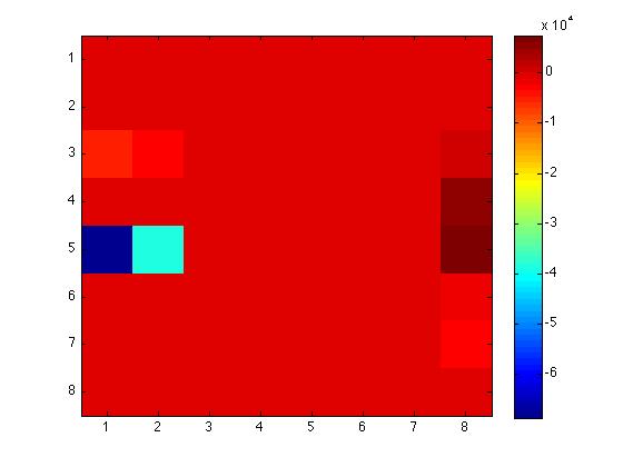 The determinant of the Jacobian is 4.6371e+04 (so I’d assume the system would blow up) except most of the entries are negative. Oh! Wait, I'm thinking of the meaning of this determinant in the wrong way! It's mapping the equilibrium state (which is at a coordinate in the 8 dim state space with all positive/zero values except for one, x) to very large negative numbers, which means the system's xdot is large and negative, which is a very good thing, meaning even the linear system is stable. I'm not sure if that was very understandable. Let me compute Jacobian(equilibrium state)*equilibrium state:
1.0e+04 *
The determinant of the Jacobian is 4.6371e+04 (so I’d assume the system would blow up) except most of the entries are negative. Oh! Wait, I'm thinking of the meaning of this determinant in the wrong way! It's mapping the equilibrium state (which is at a coordinate in the 8 dim state space with all positive/zero values except for one, x) to very large negative numbers, which means the system's xdot is large and negative, which is a very good thing, meaning even the linear system is stable. I'm not sure if that was very understandable. Let me compute Jacobian(equilibrium state)*equilibrium state:
1.0e+04 *
0
0
-0.4165
-0.0082
-5.6239
-0.0078
-0.0091
-0.0005 Yup, all good! So, how do I find the major/minor axes of the lyapunov function, so I can better understand the orientation of its level set ellipses? Ha, wait, no, I think what I really wanted was not xdot [which is, for the linear system, Jacobian(equilibrium state)*equilibrium state], but the eigenvalues of Jacobian(equilibrium state), which are indeed indicative of a stable system:
1.0e+02 *
-0.0127 + 2.0976i
-0.0127 - 2.0976i
-1.6867
-0.1205 + 0.4703i
-0.1205 - 0.4703i
-0.0000
-0.0103 + 0.1234i
-0.0103 - 0.1234i However, I just found a bug in my code: I need to be computing xtilda' S xtilda not x'Sx to determine the value of the Lyapunov function (or its time derivative) at a point, where xtilda is x-equilibrium, because otherwise, it's as if the Lyapunov function's center is at the origin of the state space, not the equilibrium! (Clearly incorrect, and probably the cause of the strange behavior earlier. Yay for bugs found!) 3.5858e+04 is the value of rho for the lyapunov candidate suggested by Matlab's lyap command when given an initial Q that is the identity. How will I visualize this? I could--wait, first I have to figure out if this experimental ROA crosses over a state-based hybrid state transition boundary. The smallest rho I could find (on the easiest boundary) was 3.0503e+04, slightly smaller than the rho found without taking boundaries into account. So, this experimental ROA was bleeding over transitions boundaries. Whoops! What about the other transition boundaries? They're based on relationships between fn and fs, which are (nontrivial?) functions of the state variables, and also on the sign of fn and fs. (Depending on what quadrant of fn, fs space you're in, your subject to a different transition boundary.) I'll pull up Alexis' paper, just to make sure I get the relationships exactly right, and then I can do the same thing I did before for the tail-on-wall-based boundary: randomly generate states on the boundary, and find the minimum rho over a sufficiently large number of sampled states. While I usually think of the visual representation of the "success/failure boundary" (switching surface for stuck-on-wall --> off-wall or sliding-on-wall), there is a representation that's a little easier for converting in to code in Table 2 of Alexis et al.'s IJRR draft: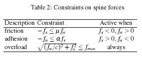 (Alexis and I didn't talk about the overload condition, and I don't think it's part of his hybrid model, but would it really hurt to include it in this particular stream of analysis? Probably not.)
What are fn and fs in terms of the state variables?
fs = (((1+(-1+(gamma*Lt+qS)^2)*sin(qH-qA-qK)^2)*(Lt*(1-gamma)*sin(qA-qH)-Lf*cos(qA-qH)-(gamma*Lt+qS)*cos(qH-qA-qK))+sin(qH-qA-qK)*cos(qH-qA-qK)*(1-(gamma*Lt+qS)^2)*(Lf*sin(qA-qH)+Lt*(1-gamma)*cos(qA-qH)-(gamma*Lt+qS)*sin(qH-qA-qK)))*( ...
(Alexis and I didn't talk about the overload condition, and I don't think it's part of his hybrid model, but would it really hurt to include it in this particular stream of analysis? Probably not.)
What are fn and fs in terms of the state variables?
fs = (((1+(-1+(gamma*Lt+qS)^2)*sin(qH-qA-qK)^2)*(Lt*(1-gamma)*sin(qA-qH)-Lf*cos(qA-qH)-(gamma*Lt+qS)*cos(qH-qA-qK))+sin(qH-qA-qK)*cos(qH-qA-qK)*(1-(gamma*Lt+qS)^2)*(Lf*sin(qA-qH)+Lt*(1-gamma)*cos(qA-qH)-(gamma*Lt+qS)*sin(qH-qA-qK)))*( ...
kHip*(qHzero-qH)-bHip*qHp)+(gamma*Lt+qS)*(cos(qH-qA-qK)*(1+(Lf*sin(qA-qH)+Lt*(1-gamma)*cos(qA-qH)-(gamma*Lt+qS)*sin(qH-qA-qK))^2)-sin(qH-qA-qK)*(Lf*sin(qA-qH)+Lt*(1-gamma)*cos(qA-qH)-(gamma*Lt+qS)*sin(qH-qA-qK))*(Lt*(1-gamma)*sin(qA- ...
qH)-Lf*cos(qA-qH)-(gamma*Lt+qS)*cos(qH-qA-qK)))*(kKnee*(qKzero-qK)-bKnee*qKp)+nSpines*(sin(qH-qA-qK)*(1+(-1+(gamma*Lt+qS)^2)*sin(qH-qA-qK)^2+(Lf*sin(qA-qH)+Lt*(1-gamma)*cos(qA-qH)-(gamma*Lt+qS)*sin(qH-qA-qK))^2)-cos(qH-qA-qK)*(sin(qH- ...
qA-qK)*cos(qH-qA-qK)-(gamma*Lt+qS)^2*sin(qH-qA-qK)*cos(qH-qA-qK)-(Lf*sin(qA-qH)+Lt*(1-gamma)*cos(qA-qH)-(gamma*Lt+qS)*sin(qH-qA-qK))*(Lt*(1-gamma)*sin(qA-qH)-Lf*cos(qA-qH)-(gamma*Lt+qS)*cos(qH-qA-qK))))*(kSpine*qS+bSpine*qSp))/((sin( ...
qH-qA-qK)*cos(qH-qA-qK)-(gamma*Lt+qS)^2*sin(qH-qA-qK)*cos(qH-qA-qK)-(Lf*sin(qA-qH)+Lt*(1-gamma)*cos(qA-qH)-(gamma*Lt+qS)*sin(qH-qA-qK))*(Lt*(1-gamma)*sin(qA-qH)-Lf*cos(qA-qH)-(gamma*Lt+qS)*cos(qH-qA-qK)))^2-(1+(-1+(gamma*Lt+qS)^2)*sin( ...
qH-qA-qK)^2+(Lf*sin(qA-qH)+Lt*(1-gamma)*cos(qA-qH)-(gamma*Lt+qS)*sin(qH-qA-qK))^2)*(sin(qH-qA-qK)^2+(gamma*Lt+qS)^2*cos(qH-qA-qK)^2+(Lt*(1-gamma)*sin(qA-qH)-Lf*cos(qA-qH)-(gamma*Lt+qS)*cos(qH-qA-qK))^2)); fn = -(((sin(qH-qA-qK)^2+(gamma*Lt+qS)^2*cos(qH-qA-qK)^2)*(Lf*sin(qA-qH)+Lt*(1-gamma)*cos(qA-qH)-(gamma*Lt+qS)*sin(qH-qA-qK))+sin(qH-qA-qK)*cos(qH-qA-qK)*(1-(gamma*Lt+qS)^2)*(Lt*(1-gamma)*sin(qA-qH)-Lf*cos(qA-qH)-(gamma*Lt+qS)*cos(qH- ...
qA-qK)))*(kHip*(qHzero-qH)-bHip*qHp)+(gamma*Lt+qS)*(sin(qH-qA-qK)*(sin(qH-qA-qK)^2+(Lt*(1-gamma)*sin(qA-qH)-Lf*cos(qA-qH)-(gamma*Lt+qS)*cos(qH-qA-qK))^2)+cos(qH-qA-qK)*(sin(qH-qA-qK)*cos(qH-qA-qK)-(Lf*sin(qA-qH)+Lt*(1-gamma)*cos(qA-qH)-( ...
gamma*Lt+qS)*sin(qH-qA-qK))*(Lt*(1-gamma)*sin(qA-qH)-Lf*cos(qA-qH)-(gamma*Lt+qS)*cos(qH-qA-qK))))*(kKnee*(qKzero-qK)-bKnee*qKp)-nSpines*(cos(qH-qA-qK)*((gamma*Lt+qS)^2*cos(qH-qA-qK)^2+(Lt*(1-gamma)*sin(qA-qH)-Lf*cos(qA-qH)-(gamma*Lt+ ...
qS)*cos(qH-qA-qK))^2)+sin(qH-qA-qK)*((gamma*Lt+qS)^2*sin(qH-qA-qK)*cos(qH-qA-qK)+(Lf*sin(qA-qH)+Lt*(1-gamma)*cos(qA-qH)-(gamma*Lt+qS)*sin(qH-qA-qK))*(Lt*(1-gamma)*sin(qA-qH)-Lf*cos(qA-qH)-(gamma*Lt+qS)*cos(qH-qA-qK))))*(kSpine*qS+ ...
bSpine*qSp))/((sin(qH-qA-qK)*cos(qH-qA-qK)-(gamma*Lt+qS)^2*sin(qH-qA-qK)*cos(qH-qA-qK)-(Lf*sin(qA-qH)+Lt*(1-gamma)*cos(qA-qH)-(gamma*Lt+qS)*sin(qH-qA-qK))*(Lt*(1-gamma)*sin(qA-qH)-Lf*cos(qA-qH)-(gamma*Lt+qS)*cos(qH-qA-qK)))^2-(1+(-1+( ...
gamma*Lt+qS)^2)*sin(qH-qA-qK)^2+(Lf*sin(qA-qH)+Lt*(1-gamma)*cos(qA-qH)-(gamma*Lt+qS)*sin(qH-qA-qK))^2)*(sin(qH-qA-qK)^2+(gamma*Lt+qS)^2*cos(qH-qA-qK)^2+(Lt*(1-gamma)*sin(qA-qH)-Lf*cos(qA-qH)-(gamma*Lt+qS)*cos(qH-qA-qK))^2));
TailPenetration = x + Ltaily*sin(qA) - Ltailx*cos(qA); Mmm... So I was able to reason a little about the "shape"/form/dimension of the tail-based switching surface before, which had such a simple description in terms of state variables. First (easiest) question to answer: do fn and fs each depend on every state variable? By inspection, both depend on qA, qH, qS, and qK. Thanks to the find function, I know that neither depend on x, xp, yp, or qAp. Let's start with the friction-based boundary, without worrying about the quadrant of fn,fs space in which it applies: -fs = μfn -fs(qA,qH,qS,qK) = μfn(qA,qH,qS,qK) 0 = μfn(qA,qH,qS,qK) + fs(qA,qH,qS,qK) I probably cannot rearrange the equation for qA in terms of qH, qS, and qK (or solve for any of the others in terms of the remaining three), so I'm going to need to numerically solve for the zero of the RHS above. I'll try Matlab's fzero function; an example of the appropriate syntax is: x = fzero(@(x)sin(x*x),x0); Making a function of the form val = fricbound(qA,qH,qS,qK), so I can call fzero on the anonymous function @(x)fricbound(x,qH,qS,qK) [or @(x)fricbound(qA,x,qS,qK) or @(x)fricbound(qA,qH,x,qK) or @(x)fricbound(qA,qH,qS,x) ], with initial value in the middle of a 2pi range of the unspecified angle. (The reason I've specified all the possible fricbound-based anonymous functions I can plug into fzero is because it's not entirely clear to me that all possible points on the friction-based transition boundary can be created by randomly sampling the same three angles and solving for the same fourth angle every time. I could randomly sample which angle is solved for.) Question: is the absolute value of these angle a factor in fn and/or fs, or just their sine and cosine? If the former is true, I couldn't just choose any arbitrary 2pi interval to sample/search. Answer: Yes, the absolute value of the angle does affect the value of fn and/or fs. So what is the correct 2pi interval to sample? The IJRR paper has labeled the plane in a way that does not obviously correspond to the state variables I have for our model, so I'm not exactly sure what qA, etc. are. Argh. Here are the terms (which occur in both fn and fs) that concern me: (gamma*Lt+qS)^2 (gamma*Lt+qS) (kSpine*qS + bSpine*qSp) kHip*(qHzero-qH) kKnee*(qKzero-qK) Oh--I assumed qS was an angle because of the qA, qK, and qH are, and are also preceded by q, but no, qS is in meters. Its initial value is 0. I wish I knew what it meant. Ah, it's the extention due to the foot, called e_s in the IJRR draft, I believe. And it probably only extends, so I'll sample randomly from 0 to 1 cm, which is a reasonable amount of extension, given my little bit of time playing with the mechanism. And I can sample +/- pi around the qHzero and qKzero to generate random qH and qK. Actually, can I limit it also by figuring out the configuration limits from the diagrams in the IJRR draft? Based on the illustration, qH and qK look like they can only vary by pi, and from 0 to pi at that, the way they're defined. qA looks like it's the angle the body of the plane makes with the wall (which is aligned with the traditional horizontal/vertical coordinate frame). I could let that vary from +/- pi (the full revolution) even though many of those configurations are unlikely... Are these dynamics valid even if the plane is, say, upside-down? Could I artificially limit the size of the level set of the lyapunov function by making it limited by nonvalid dynamics (evaluation of the dynamics function and/or the hybrid state transition boundaries outside where they are valid)? I feel like it is particularly possible for this to happen from extending the definitions of the hybrid state transition boundaries into regions of state space for which they are no longer valid. When I'm ready to generate points, if I use fzero to solve for a value, I'll have to test that it's a reasonable value (qS shouldn't be negative, I think, and qH and qK ... 1Jan2011 The following scanned pages show my thought process about random state generation for sample-based ROA verification, and how best to handle unreachable regions of the state space: Now we can generate a unit sphere of points in space B and map it to the ellipsoidal shell that is a particular level set of the lyapunov function in the state space. Very handy for our sample-based ROA approximation generation!
Also had a very productive meeting with Alexis today. We covered all the points I wrote down this morning (in the bulleted list above). Will bring this blog entry up to date with our decisions and the answers to my questions this evening.
First part of my update based on my discussion with Alexis:
We hammered out a plan. Turns out that we cannot know how conservative/appropriate the quadratic lyapunov candidates are for approximating the true ROA until Alexis runs a different script than the one that generated the landing envelope figures in his publications.
He does not have all the configuration constraints for the full model, and they're much simpler for the reduced order model, which he's currently testing to make sure it's correct.
Our plan is the following: 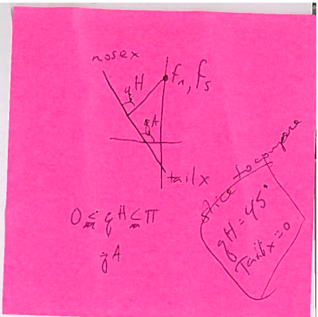 6Jan2010
This morning I woke up at sunrise and immediately finished debugging my code for using sampling to estimate the ROA. Alexis responded about a couple parameter values that would have to be the same in our respective pieces of code, and I made the appropriate parameter value changes to reflect his choices. While my code appears to be working properly, it's hard to know if there are any bugs still lurking in it because I have nothing to compare it to yet. Emailing Alexis about that now. I wonder if he's in the lab, and if his cluster has returned an ROA based on exhaustive simulation yet...
Thought a bit about how to only sample on the level set in the slice of state space defined by qH = 45 degrees, tailpenetration (or tailx?) = 0, since that's the slice Alexis is computing, but instead of a cute linear algebra solution, I tried some manipulation on the white board and decided it was easier and quicker to just sample in the space and mark with a color whether or not the point falls inside or outside the level set.
Accumulated To Do List
6Jan2010
This morning I woke up at sunrise and immediately finished debugging my code for using sampling to estimate the ROA. Alexis responded about a couple parameter values that would have to be the same in our respective pieces of code, and I made the appropriate parameter value changes to reflect his choices. While my code appears to be working properly, it's hard to know if there are any bugs still lurking in it because I have nothing to compare it to yet. Emailing Alexis about that now. I wonder if he's in the lab, and if his cluster has returned an ROA based on exhaustive simulation yet...
Thought a bit about how to only sample on the level set in the slice of state space defined by qH = 45 degrees, tailpenetration (or tailx?) = 0, since that's the slice Alexis is computing, but instead of a cute linear algebra solution, I tried some manipulation on the white board and decided it was easier and quicker to just sample in the space and mark with a color whether or not the point falls inside or outside the level set.
Accumulated To Do List
Research
5Nov2010 Skype with Russ, Mark, Alexis, Elena:- What is the current state of the model? DOF = 6 (3 plane, 3 legs). Look now at upward sliding along wall with Coulomb friction.
- Seems good to do 6 + elevator. After detachment, legs slowly relax back to equilibrium position.
- Legs essentially massless, so have 1st order dynamics while free -- essentially need a timer to know how long it takes for legs to get back to equilibrium position.
- Leg hits wall, there is some discontinuity in force due to damping in the leg (spring force ramps smoothly).
- Unliateral constraint of staying attached + slipping. Need plane momentum to be sufficient to stay in contact with wall, and then look for whether vertical velocity can reverss ==> attachment, or whether you instead bounce off.
- Shows the normal and shear forces over time for the last of ~200 simulations from various initial x and y velocities:
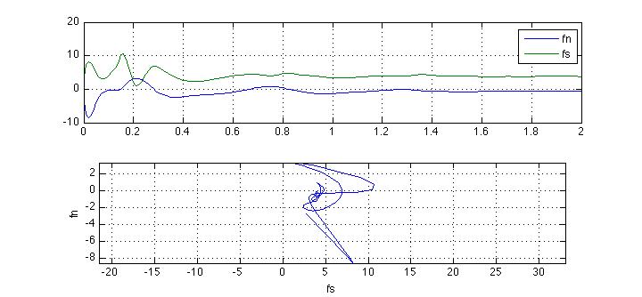
- Shows the normal and shear forces at the last computed moment in time for all ~200 simulations:
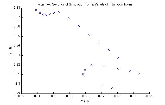
- I only need to simulate from one initial condition (for a "long" time) to get the equilibrium, because there's only one, in terms of the variables we care about. (I guess I was trying a bank of different initial conditions because I thought I'd make sure there was only one....)
- Yesterday Alexis and I thought we discussed covering the landing envelope with several ellipses, about different linearization points, in order to cover the region less conservatively. By landing envelope, we mean the region in xdot, ydot of the foot at touchdown from which the plane does ultimately reach its static equilibrium. This is correct, but needed further detail to make it fully representative of what's involved. While we can linearize the dynamics at any point in the state space, region of attraction to a linearization point only makes sense when that linearization point is also a fixed point (a static equilibrium). Regions of attraction around non-fixed points are regions of attraction to a trajectory. Therefore the linearization points and ellipsoids plotted in the foot-xdot,-ydot-at-touch-down space represent the projections of points along and regions of attraction around trajectories that lead to the static equilibrium point.
- Alexis' initial conditions were fine if the thruster came on, but did not produce a static equilibrium. He readjusted them after I pointed this out. I should have been able to do this myself, but I thought it might have been the result of an error or problem with the model when simulated on my machine as opposed to his (stranger things have happened before!). And the axes of the plot of the plane's state overtime were not set to "equal" thus making it hard to see what was actually happening.
- Matlab just finished simulating a long run in which the static equilibrium was reached, which is now saved in the automatically generated output files. Better not overwrite them by any subsequent runs of the code before saving the results more permanently! After that... Next step, linearization!
- The hip stiffness calculating function that was giving me trouble last night turns out to have logic within it, so that it implements a function that is non-differentiable at a point; it's got a "kink" at the transition between a curve and a plateau. At first, not being differentiable at one point seemed to be okay to me, with respect to taking gradients... What's the likelihood that you land on the point where the function is undefined? In theory-land, zero. However, we're finding gradients symbolically, and that kind of function, which is piecewise, requires the gradient equations to have logic within them, and I don't think our gradient-function-generating code does that. Therefore Alexis and I concluded that piecewise dynamics, and also any logic at all which we subsequently found within the dynamics function just for sticking (tail and nose penetration boolean variables, for example), mean that what we thought was one model of a larger hybrid model is itself a hybrid model. We'd chosen to model the contact of the tail and nose with the wall as spring-damper systems, because it meant Alexis could use one call to MotionGenesis? to generate the dynamics, and we thought it would reduce the number of hybrid states, but it doesn't! We got rid of the logic within the sticking state so that both MotionGenesis? and my gradient generating code can handle it, and of course, since the logic was gone, we hardcoded the boolean variables to be the values they'd be at the static equilibrium we're going to evaluate the gradients at. So it's nice that these gradients are symbolic, but they're only valid for the regions in which these hardcoded boolean values are correct. We may have a lot of different gradient functions (and therefore a lot of states in our hybrid system) by the time we're done!
- If our equlibrium point is very close to the edge of the hybrid state it is in, will that interfere with the expansion of our conservative region of attraction estimates? Can a region of attraction calculated with SOS "bleed" over into another hybrid state, across a state transition? I'm going to email Russ and Mark T about that now. It's too interesting not to.
If a trajectory ended in the ROA of an existing trajectory, but not on the trajectory, then the ROA for the endpoint of that new trajectory would be smaller (I'm pretty sure) than if it had ended on the existing trajectory, since the ROA of the endpoint of the new trajectory has to fall entirely within the ROA of the trajectory it's feeding in to.
Also, if an optimizer like SNOPT has found a trajectory endpoint in the ROA of an existing trajectory, how much "harder" could it be to add some time to the new trajectory and actually connect it to the existing trajectory?
Note: the ultimate connection point may be at a point "far downstream" of the trajectory waypoint whose associated ROA the endpoint initially fell in to. I guess, to be technically correct, I should say funnel time-slice, rather than ROA of a trajectory waypoint, because the latter terminology suggests that points in that waypoint "ROA" will go to that waypoint, rather than thinking of the ROA as the slice of a funnel in which all trajectories approach the associated nominal trajectory.
The fact that we're considering purely passive trajectories [we are not steering the plane toward existing trajectories] suggests that trajectories that connect back to the tree would all connect at the static equilibrium (root tree node).
So, it looks like we have two choices in terms of tree structure, depending on whether or not we force new trajectories to connect back to tree or just let them end somewhere in the funnel of an existing trajectory (perhaps with a preference for a location nearer, rather than farther, to the center of that funnel): if we choose the former option, we might get a spaghetti-like structure all coming out of the static equilibrium, and if we choose the latter option, we might get more of a tree-like structure, with branches coming off of branches, but with possibly thinner funnels. Remaining progress to report on:
- Elaborating on my refined understanding of time invariant and finite horizon time (passive) ROAs for (passive) trajectories, which I started to do above but did not finish.
- Russ & Mark T's responses to my questions about ROAs and hybrid system transitions
- Alexis' progress, which will shortly be followed by my progress, on A, B generation of xdot = Ax + Bu for the static equilibrium, which includes Alexis' awesome automatic model generator using a pre-processor macro in Aquamacs.
- Possibly: the connection between hybrid systems and the discussion of jump linear dynamical systems in Boyd's EE263
Also, we need at least second order terms for the Taylor expansion of the dynamics, because the friction model is of just Coulomb friction, and the high slope of the Coulomb friction approximation at the linearization point is going to adversely affect the accuracy of the Taylor approximation a LOT unless there are higher order terms to capture its plateaus. We could leave out the friction term, but then the resulting ROA would be for the frictionless model; there's no control on which to tag a feedforward model of the friction--oh wait!! What if our "passive controller" for the TI ROA calculation was just the forces from the friction model? Would that make sense? I'm not sure which is better/more accurate: calculating a high order Taylor expansion of the dynamics and calculating the TI ROA with no input or calculating a less high order Taylor expansion of the frictionless dynamics and calculating the TI ROA for a controller which is actually just imposing the forces from the friciton model.
Since Alexis can generate the same symbolic gradients I'm trying to generate with the generate_dynamics_func_gradients (but doesn't package them like our code does), and I am not getting traction on what is most likely a memory issue with our code, I think we'll have to write a script to use Alexis' MotionGenesis? to generate the first, second, and perhaps third order terms of the Taylor series, which will of course be high-dimensional tensors.
For now (today) I think I'll calculate the TI ROA with a first order Taylor expansion of the frictionless dynamics, using a "controller" which is actually just imposing the forces from the friciton model.
22Nov2010 Getting Back on Track
Somehow, it feels like progress has slowed to a crawl, and I'm not sure why. Well, actually, I do know why, and it's that things are taking longer to calculate than exp I think it's time to step back, survey the situation, the goals, and the differences between perceived and actual calculation difficulties in order to decide the best next steps. Some "data points:"
- When I attempted calculating A on my own laptop, Matlab had gotten, well, it's not entirely clear how far it got, because some of A's entries were so large they pushed the rest over the threshold that Matlab will print out in the command window. Anyway, after two days, my entire laptop froze to a halt. I should have been saving the A matrix after each entry was calculated, not after the whole thing was calculated. My mistake! However, there must be a more efficient way to do this. It's trivially parallelizable. Can I send it off to the Matlab cluster to be computed in parallel? That would be the only way to get the higher derivatives too.
- It's not like I was sitting at my desk, watching Matlab hum along. I was trying to figure out whether it was better to (1) find an ROA for the dynamics including friction, which would require many more higher order terms in the Taylor expansion than the frictionless dynamics in order to get similar accuracy over similar distances from the linearization point or (2) find the ROA for the dynamics w/o friction and assume we can cancel the friction out with a feedforward term based on the friction model [Alexis reminded me that since this friction acts at an unactuated "joint"--the contact point between the tail and the wall--we cannot, in reality, cancel out that friction with a feedforward term applying forces at that joint. However, is it possible to compensate for that friction with forces at an actuated joint, like non-collated control? ] (3) find the ROA for the dynamics w/o friction and assume friction is inconsequential, as Alexis suggests it is. It may be inconsequential in the hybrid model that we're considering, in which the static equilibrium for being stuck on the wall exists, but it won't be inconsequential in the future, so it's good, at least, that we spent some time thinking about its incorporation, even if we do end up ignoring it for the purpose of calculating our first ROA.
- Next steps: see if I can get the symbolic A, B from Alexis' code, or better understand why he said it was way easier to get numerical values, not the full symbolic matrices, and look into parallelizing the computation of A, B, and the higher order derivatives and running it on a cluster at MIT or Stanford.
I think the true reason my progress has become more labored is that I'd lost sight of the ultimate cool things I want to create/make possible, and they are:
- A flapping-wing DAV that flits around the Robot Locomotion Group Lab space, and lands on the specially-outfitted gloved hand of any visitor who'd like to have a robotic bird perch on them.
- Tool(s) to help mechanical designers expand ROAs by trial and error modification of the mechanics and ROA calculation using SOS.
The first bullet point is so far away that, while it's fun to briefly day-dream about, it doesn't seem to have much function as far as guiding my immediate next steps. The second one came up in the course of conversation with Alexis since I've been here, and is what I'm currently working on. While it is important to get things going for our specific model, it's not unreasonable to also consider how best to generalize it, or what computational issues others might run in to if they tried it themselves. (Is it only practical if you have access to a computer with _ amount of memory, or if you have the Matlab Parallel Computing Toolbox?)
After looking at Tig's info on distributed computing (sending jobs to our CSAIL cluster) and realizing that it looked like there was some nontrivial start-up costs in terms of time/effort, I asked Noe if he'd used a cluster here at Stanford. He showed me how to log in to a server (ssh -X corn.stanford.edu -l $SUNETid) and start up matlab remotely, while tunnelling the graphics to my local machine. Pretty neat! I'm curious to see how much faster it is to compute a couple of the A and B matrix entries, but I also am still very interested in ultimately parallelizing it.
23Nov2010 I <3 Sending Jobs to Powerful Servers Somewhere Else
No parfor or matlabpool commands necessary. Installing Fetch, using it to put Robotlib in my AFS space, X-tunnelling to corn.stanford.edu, starting Matlab, installing (running configure) Robotlib within Matlab on the server, and executing the commands that froze my laptop. And it's ripping through the calculations! But still taking long enough that I'll need to go to bed and check on it in the morning. DEFINITELY need to use parfor, especially for higher order derivatives of the dynamics.
Other accomplishments for the day:
- talking to multiple MIT secretaries about financial matters
- talking to Stanford Health and Student Support Services to resolve a billing mistake
- Working on EE263
24Nov2010 Servers Aren't Supercomputers
Well, like the title of my "blog post" implies, servers aren't supercomputers, and A is still being calculated. It's been running all night (about 8 hours). It's gotten much farther, more quickly, than when the code runs on my computer. LUCKILY, I'm saving every time an entry of A is calculated, and even if Matlab hangs up and becomes unresponsive, I can still use Fetch to retrieve what of A has been calculated. There is, however, a wrinkle. If I evaluate A (a 1.6 MB array after just one hour of calculations) in my local copy of matlab, I cannot open it in the variable editor. Matlab gets stuck. And I can evaluate A at the command line, but then I only see part of it because Matlab doesn't print out the right side of print-outs that are more than some threshold of characters wide. After 11 hours of computation on the server, it's 7 MB large. Oh, it just finished!! Halleluyah! I have my symbolic A matrix!!! Saved! And backed up in two places! Now, to calculate B. Projected completion time, if the relationship between xdot and the input is of comparable complexity: (11hrs/9)*2 inputs. Actually, I don't even need to compute that, since we're looking at passive ROAs first. Awesome! Finally! What a relief. I was in the middle of writing an email to the folks back home in the RLG and Tig about how to submit jobs to our CSAIL cluster (which is the only way to go, it seems, for higher order derivatives), so while that need is less urgent, I'll still send the email.
Now, to calculate B. Projected completion time, if the relationship between xdot and the input is of comparable complexity: (11hrs/9)*2 inputs. Actually, I don't even need to compute that, since we're looking at passive ROAs first. Awesome! Finally! What a relief. I was in the middle of writing an email to the folks back home in the RLG and Tig about how to submit jobs to our CSAIL cluster (which is the only way to go, it seems, for higher order derivatives), so while that need is less urgent, I'll still send the email. Leaving now for the office, where I can work on steps 3 and 4 from November 8th. First step: creating the file which spells out A, automatically, in the way the rest of the tools expect it, and is automatically generated from the symbolic A matrix I produced overnight last night. This file allows me to see each A matrix entry, which cannot be done in the usual way in the variable editor due to A's size. In fact, it allowed me to see that I'd made a one character mistake in my A-generating code, and now need to rerun the code overnight tonight. Darn! [29,30]Nov2010 Feeling a Tad Silly Yesterday, Alexis and I were both back from Thanksgiving break, and talking face to face about our bottlenecks. Memory available on the machine, how many processors were recruited for parallelized tasks, constraints on the parallel version of a for loop in Matlab, memory limits imposed by what license we have for Motion Genesis, Motion Genesis' "auto-z" function which helps reduce computational [time? memory?] needs, Matlab's switch from Maple to Mupad... were all discussed. I told Alexis that it took 11 hours to compute the symbolic Jacobian of the hybrid state of being stuck on the wall (the one we've been working with, primarily). "That's weird," he replied. With a few keystrokes, he executed a differentiation of the dynamics with respect to our state variables. Two seconds later, the command line prompt returned. "Done! That's the A matrix!" he informed me, and I could see that, of course, it was, but the statement computing each of the entries of the symbolic Jacobian looked unfamiliar. "Wait... no...! But...?!?" is a pretty good representation of my response. "Something is wrong here. Let me grab my laptop and show you my code. I need to understand what's going on here." I ran back to CDR to grab my computer. Back in the lab, I beckoned him to look glance at my code. It was not obvious why his would execute so quickly and mine would execute at a snail's pace--a pace unworkably slow. However, there was a clue. It took 15 minutes to display a single element of the symbolic Jacobian, and he mentioned that it crashed his computer occasionally. Fifteen minutes just for typing A(i,j) at the command line and hitting enter. My guess is that his alternative way of submitting arguments to the symbolic diff command sidestepped "thinking" about A(i,j) in the same way Matlab does when you type it into the command line and hit enter. Unfortunately, in order to write the file of gradients that our toolbox expects, it currently evaluates each A(i,j) in the way Matlab does at the command line. Last night I was thinking about how to get around that, but I think instead I'll just save a mat containing "df" (which is a struct containing the first, second, third, etc. order derivatives of the dynamics) and have that load into a persistent variable (so it's only loaded once). There is something really weird about all this, and after I get the next stuff going, I need to figure it out. It could have serious implications about other uses of Matlab's symbolic capabilities in our group. If it's this easy to write code that does the same thing, in two very simple ways, in which one takes many orders of magnitude longer to run, it's important that people (and I) understand the quicker, equivalent way to write it. ALSO the gradient-generating code in our Robotlib toolbox should be rewritten, in light of this information, because that's the ultra-slow code I was using! Another word of caution: code later on down the line will need to work with A(i,j), so hopefully we can figure out how to do that stuff as well without needing to suffer that significant time penalty. Here are some of the basics: Alexis' quick differentiation code:Hi Tig!
Well, this is embarrassing to admit, but after reading the how-to info on the Tig Wiki, I am still unclear as to how to submit jobs to our cluster. I'm not even sure if submitting jobs to the cluster would solve my computing problems!
Here's a description of my problem:
It took 11 hours on a server to produce a 9x9 symbolic matrix in Matlab, whose entries are symbolic derivatives of a complex symbolic function. The whole matrix is 7 MB large. When I ran the same code on my own laptop, it crashed my machine after not getting very far over 2 solid days of crunching. I think Matlab may have some memory leaks, but there's not much I can do about that (I think).
11 hours is almost okay, except for the fact that I'd like to compute a 9x9x9 symbolic matrix of second order derivatives, which may be of similar complexity. If this takes 9 times as long, my current method of running jobs on the server is not practical.
This job is trivially parrallelizable. However it's unclear to me whether computational or memory limitations of the server I'm using are holding me back, or if the Condor cluster would offer a speed-up in this case.
Any thoughts? If the cluster is appropriate, I still don't seem to have enough background in order to understand how to submit my job. Yikes! (And yes, this is my 7th year here at MIT. Yes, I should know this. But I took advanced math and circuits and signal processing classes, not CS classes that would have taught me this kind of stuff, so now I feel a tad helpless and silly. At least I can say that if you had a radio from the 1940's, I could fix and restore it. Haha. :-P
Cheers,
Elena
syms"char(statesderivatives(i))" is, by the way, unnecessarily "wordy;" it can be replaced with "statesderivatives{i}," since the contents of that cell in the state derivatives cell array is of type char. Indexing into an array using curly braces extracts the contents of the cell at the index; indexing into the array using parentheses gives you the cells that contain the contents at the index. After playing around with various things, I've determined that it takes at most a couple seconds to differentiate one of the state derivatives with respect to a state if the result is not printed to the screen. Leave off the semicolon at the end of the line and Matlab will get back to you, but not before you've returned from a long, slow walk through the park. (That's a joke--I have not gone for walks while waiting for it. Alexis told me it would take 15 min or so. And I stop it after two minutes, max.) When Dealing with Symbolsxp = yp = .... states = {'x' 'y' 'qA' 'xp' 'yp' 'qAp' 'qH' 'qK' 'qS'};
statesderivatives = {'xp' 'yp' 'qAp' 'xpp' 'ypp' 'qApp' 'qHp' 'qKp' 'qSp'};
for i = 1:9
tic
for j = 1:9
A(i,j) = diff(eval(char(statesderivatives(i))),char(states(j)));
end
disp(i)
toc
end
- Do not print out the result of a calculation, like diff. The diff command will take a couple seconds, at most, to do its job. Printing out the result will take as much as 15 min or more. So will printing out any particularly long entires of a symbolic matrix.
- Do not apply the command "simple" to these complicated entries. It's not worth the incredibly long time it will take to perform simplifications, if any even exist.
- Do not attempt to save a symbolic matrix with complex entries. This will take forever. If you use ctrl-c to stop it, you'll have to press it down many many times, and for each repetition, Matlab spits out something of this form:
Warning: Error saving an object of class 'sym':
Error using ==> mupadengine.mupadengine>mupadengine.evalin at
123
-1/IzzAirplane*(cos(x2 - x1 - x3)/(((cos(x2 - x1 - x3)Error:
Computation aborted - Do not attempt to write a complicated symbolic matrix to a file. This will take forever. If you use ctrl-c to stop it, you'll see something of this form:
??? Operation terminated by user during ==>
mupadengine.mupadengine>mupadengine.evalin at 117
In ==> mupadsym.mupadsym>mupadsym.char at 30
s = evalin(symengine,x.ref,'char');
In ==> sym.char at 18
M = char(A.s);
In ==>
generate_dynamics_func_gradients_BDML>write_symbolic_matrix at
123
for i=1:m, for j=1:n, if (A(i,j)~=0) fprintf(fp,'a(%d,%d)
= %s;\n',i,j,char(A(i,j))); end; end; end
In ==> generate_dynamics_func_gradients_BDML at 89
write_symbolic_matrix(fp,df{1},'df{1}');
And my last attempt at finding the Jacobian turns out to have given me a matrix of NaN? . We'll have our more powerful version of MotionGenesis? up and running soon, so this seems like an appropriate time to put my classwork-hat back on.
[2,3]Dec2010 Not Just Describing the Symptoms, but Understanding the Underlying Phenomena
Suddenly, memory (virtual, physical, swap files, etc.) management has become very interesting! I've found the following pages helpful: [not an exhaustive list] - http://6004.csail.mit.edu/
- http://www.mathworks.com/support/tech-notes/1100/1107.html
- http://www.mathworks.com/support/tech-notes/1100/1106.html?BB=1
- http://www.mathworks.com/company/newsletters/news_notes/june07/patterns.html
Solve for a quadratic Lyapunov candidate using the following command in Matlab: S = lyap(A',eye(n)), where n is the number of statesA is pretty big, but let's see if this works... Ha. After 15 minutes, Matlab yelled at me in the following way: ??? Error using ==> lyap at 36
The input arguments of the "lyap" command must be numeric arrays. I was just feeding it the symbolic A! Silly me. Will evaluate A at the equilibrium point, with all the model parameter values substituted in. I can do this one of two ways: (1) work on the auto-generated gradients .m file, since that can be used to spit A out with everything substituted in or (2) sub things in myself using subs commands, etc. I prefer option 1, since that's how it'll be done in the robotlib code. However, Matlab won't let me use its editor, because the file's too big, and XCode, which I was using before, just crashed. Aquamacs was recommended online for working with large text files on a Mac. Installing it now. Opens it up; doesn't freeze up. Way to go, Aquamacs, you're the... program? :-P By the way, Aquamacs installation: drag icon to the Applications folder. Done. Traditional GNU Emacs installation? Run configure. Browse error messages. Apend commands to configure command and re-run. Then make. Then make install. Then... it refuses to open. Why the long, drawn-out (failed) install process when another program can do it so cleanly? Grr. Now I need to evaluate the Jacobian at the static equilibrium point, right? Yes. The equilibrium point of the linearized dynamics or the nonlinear dynamics? Shouldn't those two points be the same, if the system is started from an initial condition close enough to the goal? The friction terms have been removed; what does that mean for this particular hybrid state? The friction term(s) Alexis left out of the hybrid state I'm working on right now are not "active" at the static equilibrium because it's just the friction between the tail and the wall and is zero when the system is at rest. Fixed the script that produces the .m file of gradients based on the symbolic derivatives (which saves us the time consuming step of using slow symbolic toolbox functions like subs, etc.) and talked to Alexis. The rest point Alexis found by numerical simulation: x y qa qH qK qS x' y' qa' qH' qK' qS'
(m) (m) (deg) (deg) (deg) (m) (m/s) (m/s) (deg/s) (deg/s) (deg/s) (m/s) -1.077673E-01 -9.706154E-02 9.434811E+01 1.069099E+02 9.138784E+01 1.145137E-03 -2.475994E-08 5.670911E-09 1.213560E-06 5.527654E-06 -2.378733E-06 4.361853E-09 Packaging that up in to the state vector: [qA; qH; qK; qS; x; y; qAp; xp; yp] = [9.434811E+01; 1.069099E+02; 9.138784E+01; 1.145137E-03; -1.077673E-01; -9.706154E-02; 1.213560E-06; -2.475994E-08; 5.670911E-09] I'll plug that into the dynamics function that computes the state derivative for given state, and confirm that this is indeed a static equilibrium for the model I packaged into a robotlib plant object. Whoops! The code used to find the Jacobian has a different ordering of the variables than in the robotlib plant object. I'll multiply A by a row-switching matrix, then a column switching matrix, to make it match the robotlib plant. Is that easier than changing the robotlib plant? Nope. Changing plant now. Order consistent with Alexis' Jacobian:
state = {'x' 'y' 'qA' 'xp' 'yp' 'qAp' 'qH' 'qK' 'qS'};New static equilibrium state vector: [x; y; qA; xp; yp; qAp; qH; qK; qS ] = [-1.077673E-01; -9.706154E-02; 9.434811E+01; -2.475994E-08; 5.670911E-09; 1.213560E-06; 1.069099E+02; 9.138784E+01; 1.145137E-03] Darn, that does not produce a static equilibrium of my local plant object, and it should. What's going on? How will I debug this? I need to visualize it using Alexis' code, except it actually looks easier (and more fool-proof, from a debugging standpoint) to add a plot function directly to the plant object. I can model it on the plot function for Rick Cory's plane, but use the markers from Alexis' plot function. Actually, the plotting functions I have from him are not really what I want. I want that visualization of the plane, not just a plot of various state values over time... Will go find him... and he's gone. Time for me to go home too. Plan for tonight/tomorrow:
statederivative = {'xp' 'yp' 'qAp' 'xpp' 'ypp' 'qApp' 'qHp' 'qKp' 'qSp'};
- Copy and paste Rick Cory's plotting function into Alexis' model's plant object code.
- Make sure the (different) state variables of Rick's plane model are made to reflect the state variables of Alexis' model.
- Run simulate, with plotting. (I don't need to use LCM of course. I can use the playback function on the stored trajectory.)
- Found Rick's Glider example, got it up and running.
- Copying it into the plant object for Alexis' plane. Nope, wrong! Created a visualizer! Rick's talon will become the end of Alexis' leg, but since the leg moves with respect to the CG of the plane, it'll have to be handled a little differently than the talon its replacing in the code. Before I go any further, I realized that I was evaluating the full nonlinear (no friction) dynamics at the state vector Alexis gave me, using the plant object. Fine. But what about evaluating the Jacobian at the point that supposed to be the stable equilibrium? If that also produces large values, that will help me figure out what's wrong.
Research
5Nov2010 Skype with Russ, Mark, Alexis, Elena:- What is the current state of the model? DOF = 6 (3 plane, 3 legs). Look now at upward sliding along wall with Coulomb friction.
- Seems good to do 6 + elevator. After detachment, legs slowly relax back to equilibrium position.
- Legs essentially massless, so have 1st order dynamics while free -- essentially need a timer to know how long it takes for legs to get back to equilibrium position.
- Leg hits wall, there is some discontinuity in force due to damping in the leg (spring force ramps smoothly).
- Unliateral constraint of staying attached + slipping. Need plane momentum to be sufficient to stay in contact with wall, and then look for whether vertical velocity can reverss ==> attachment, or whether you instead bounce off.
- Shows the normal and shear forces over time for the last of ~200 simulations from various initial x and y velocities:
- Shows the normal and shear forces at the last computed moment in time for all ~200 simulations:
- I only need to simulate from one initial condition (for a "long" time) to get the equilibrium, because there's only one, in terms of the variables we care about. (I guess I was trying a bank of different initial conditions because I thought I'd make sure there was only one....)
- Yesterday Alexis and I thought we discussed covering the landing envelope with several ellipses, about different linearization points, in order to cover the region less conservatively. By landing envelope, we mean the region in xdot, ydot of the foot at touchdown from which the plane does ultimately reach its static equilibrium. This is correct, but needed further detail to make it fully representative of what's involved. While we can linearize the dynamics at any point in the state space, region of attraction to a linearization point only makes sense when that linearization point is also a fixed point (a static equilibrium). Regions of attraction around non-fixed points are regions of attraction to a trajectory. Therefore the linearization points and ellipsoids plotted in the foot-xdot,-ydot-at-touch-down space represent the projections of points along and regions of attraction around trajectories that lead to the static equilibrium point.
- Alexis' initial conditions were fine if the thruster came on, but did not produce a static equilibrium. He readjusted them after I pointed this out. I should have been able to do this myself, but I thought it might have been the result of an error or problem with the model when simulated on my machine as opposed to his (stranger things have happened before!). And the axes of the plot of the plane's state overtime were not set to "equal" thus making it hard to see what was actually happening.
- Matlab just finished simulating a long run in which the static equilibrium was reached, which is now saved in the automatically generated output files. Better not overwrite them by any subsequent runs of the code before saving the results more permanently! After that... Next step, linearization!
- The hip stiffness calculating function that was giving me trouble last night turns out to have logic within it, so that it implements a function that is non-differentiable at a point; it's got a "kink" at the transition between a curve and a plateau. At first, not being differentiable at one point seemed to be okay to me, with respect to taking gradients... What's the likelihood that you land on the point where the function is undefined? In theory-land, zero. However, we're finding gradients symbolically, and that kind of function, which is piecewise, requires the gradient equations to have logic within them, and I don't think our gradient-function-generating code does that. Therefore Alexis and I concluded that piecewise dynamics, and also any logic at all which we subsequently found within the dynamics function just for sticking (tail and nose penetration boolean variables, for example), mean that what we thought was one model of a larger hybrid model is itself a hybrid model. We'd chosen to model the contact of the tail and nose with the wall as spring-damper systems, because it meant Alexis could use one call to MotionGenesis? to generate the dynamics, and we thought it would reduce the number of hybrid states, but it doesn't! We got rid of the logic within the sticking state so that both MotionGenesis? and my gradient generating code can handle it, and of course, since the logic was gone, we hardcoded the boolean variables to be the values they'd be at the static equilibrium we're going to evaluate the gradients at. So it's nice that these gradients are symbolic, but they're only valid for the regions in which these hardcoded boolean values are correct. We may have a lot of different gradient functions (and therefore a lot of states in our hybrid system) by the time we're done!
- If our equlibrium point is very close to the edge of the hybrid state it is in, will that interfere with the expansion of our conservative region of attraction estimates? Can a region of attraction calculated with SOS "bleed" over into another hybrid state, across a state transition? I'm going to email Russ and Mark T about that now. It's too interesting not to.
If a trajectory ended in the ROA of an existing trajectory, but not on the trajectory, then the ROA for the endpoint of that new trajectory would be smaller (I'm pretty sure) than if it had ended on the existing trajectory, since the ROA of the endpoint of the new trajectory has to fall entirely within the ROA of the trajectory it's feeding in to.
Also, if an optimizer like SNOPT has found a trajectory endpoint in the ROA of an existing trajectory, how much "harder" could it be to add some time to the new trajectory and actually connect it to the existing trajectory?
Note: the ultimate connection point may be at a point "far downstream" of the trajectory waypoint whose associated ROA the endpoint initially fell in to. I guess, to be technically correct, I should say funnel time-slice, rather than ROA of a trajectory waypoint, because the latter terminology suggests that points in that waypoint "ROA" will go to that waypoint, rather than thinking of the ROA as the slice of a funnel in which all trajectories approach the associated nominal trajectory.
The fact that we're considering purely passive trajectories [we are not steering the plane toward existing trajectories] suggests that trajectories that connect back to the tree would all connect at the static equilibrium (root tree node).
So, it looks like we have two choices in terms of tree structure, depending on whether or not we force new trajectories to connect back to tree or just let them end somewhere in the funnel of an existing trajectory (perhaps with a preference for a location nearer, rather than farther, to the center of that funnel): if we choose the former option, we might get a spaghetti-like structure all coming out of the static equilibrium, and if we choose the latter option, we might get more of a tree-like structure, with branches coming off of branches, but with possibly thinner funnels. Remaining progress to report on:
- Elaborating on my refined understanding of time invariant and finite horizon time (passive) ROAs for (passive) trajectories, which I started to do above but did not finish.
- Russ & Mark T's responses to my questions about ROAs and hybrid system transitions
- Alexis' progress, which will shortly be followed by my progress, on A, B generation of xdot = Ax + Bu for the static equilibrium, which includes Alexis' awesome automatic model generator using a pre-processor macro in Aquamacs.
- Possibly: the connection between hybrid systems and the discussion of jump linear dynamical systems in Boyd's EE263
Also, we need at least second order terms for the Taylor expansion of the dynamics, because the friction model is of just Coulomb friction, and the high slope of the Coulomb friction approximation at the linearization point is going to adversely affect the accuracy of the Taylor approximation a LOT unless there are higher order terms to capture its plateaus. We could leave out the friction term, but then the resulting ROA would be for the frictionless model; there's no control on which to tag a feedforward model of the friction--oh wait!! What if our "passive controller" for the TI ROA calculation was just the forces from the friction model? Would that make sense? I'm not sure which is better/more accurate: calculating a high order Taylor expansion of the dynamics and calculating the TI ROA with no input or calculating a less high order Taylor expansion of the frictionless dynamics and calculating the TI ROA for a controller which is actually just imposing the forces from the friciton model.
Since Alexis can generate the same symbolic gradients I'm trying to generate with the generate_dynamics_func_gradients (but doesn't package them like our code does), and I am not getting traction on what is most likely a memory issue with our code, I think we'll have to write a script to use Alexis' MotionGenesis? to generate the first, second, and perhaps third order terms of the Taylor series, which will of course be high-dimensional tensors.
For now (today) I think I'll calculate the TI ROA with a first order Taylor expansion of the frictionless dynamics, using a "controller" which is actually just imposing the forces from the friciton model.
22Nov2010 Getting Back on Track
Somehow, it feels like progress has slowed to a crawl, and I'm not sure why. Well, actually, I do know why, and it's that things are taking longer to calculate than exp I think it's time to step back, survey the situation, the goals, and the differences between perceived and actual calculation difficulties in order to decide the best next steps. Some "data points:"
- When I attempted calculating A on my own laptop, Matlab had gotten, well, it's not entirely clear how far it got, because some of A's entries were so large they pushed the rest over the threshold that Matlab will print out in the command window. Anyway, after two days, my entire laptop froze to a halt. I should have been saving the A matrix after each entry was calculated, not after the whole thing was calculated. My mistake! However, there must be a more efficient way to do this. It's trivially parallelizable. Can I send it off to the Matlab cluster to be computed in parallel? That would be the only way to get the higher derivatives too.
- It's not like I was sitting at my desk, watching Matlab hum along. I was trying to figure out whether it was better to (1) find an ROA for the dynamics including friction, which would require many more higher order terms in the Taylor expansion than the frictionless dynamics in order to get similar accuracy over similar distances from the linearization point or (2) find the ROA for the dynamics w/o friction and assume we can cancel the friction out with a feedforward term based on the friction model [Alexis reminded me that since this friction acts at an unactuated "joint"--the contact point between the tail and the wall--we cannot, in reality, cancel out that friction with a feedforward term applying forces at that joint. However, is it possible to compensate for that friction with forces at an actuated joint, like non-collated control? ] (3) find the ROA for the dynamics w/o friction and assume friction is inconsequential, as Alexis suggests it is. It may be inconsequential in the hybrid model that we're considering, in which the static equilibrium for being stuck on the wall exists, but it won't be inconsequential in the future, so it's good, at least, that we spent some time thinking about its incorporation, even if we do end up ignoring it for the purpose of calculating our first ROA.
- Next steps: see if I can get the symbolic A, B from Alexis' code, or better understand why he said it was way easier to get numerical values, not the full symbolic matrices, and look into parallelizing the computation of A, B, and the higher order derivatives and running it on a cluster at MIT or Stanford.
I think the true reason my progress has become more labored is that I'd lost sight of the ultimate cool things I want to create/make possible, and they are:
- A flapping-wing DAV that flits around the Robot Locomotion Group Lab space, and lands on the specially-outfitted gloved hand of any visitor who'd like to have a robotic bird perch on them.
- Tool(s) to help mechanical designers expand ROAs by trial and error modification of the mechanics and ROA calculation using SOS.
The first bullet point is so far away that, while it's fun to briefly day-dream about, it doesn't seem to have much function as far as guiding my immediate next steps. The second one came up in the course of conversation with Alexis since I've been here, and is what I'm currently working on. While it is important to get things going for our specific model, it's not unreasonable to also consider how best to generalize it, or what computational issues others might run in to if they tried it themselves. (Is it only practical if you have access to a computer with _ amount of memory, or if you have the Matlab Parallel Computing Toolbox?)
After looking at Tig's info on distributed computing (sending jobs to our CSAIL cluster) and realizing that it looked like there was some nontrivial start-up costs in terms of time/effort, I asked Noe if he'd used a cluster here at Stanford. He showed me how to log in to a server (ssh -X corn.stanford.edu -l $SUNETid) and start up matlab remotely, while tunnelling the graphics to my local machine. Pretty neat! I'm curious to see how much faster it is to compute a couple of the A and B matrix entries, but I also am still very interested in ultimately parallelizing it.
23Nov2010 I <3 Sending Jobs to Powerful Servers Somewhere Else
No parfor or matlabpool commands necessary. Installing Fetch, using it to put Robotlib in my AFS space, X-tunnelling to corn.stanford.edu, starting Matlab, installing (running configure) Robotlib within Matlab on the server, and executing the commands that froze my laptop. And it's ripping through the calculations! But still taking long enough that I'll need to go to bed and check on it in the morning. DEFINITELY need to use parfor, especially for higher order derivatives of the dynamics.
Other accomplishments for the day:
- talking to multiple MIT secretaries about financial matters
- talking to Stanford Health and Student Support Services to resolve a billing mistake
- Working on EE263
24Nov2010 Servers Aren't Supercomputers
Well, like the title of my "blog post" implies, servers aren't supercomputers, and A is still being calculated. It's been running all night (about 8 hours). It's gotten much farther, more quickly, than when the code runs on my computer. LUCKILY, I'm saving every time an entry of A is calculated, and even if Matlab hangs up and becomes unresponsive, I can still use Fetch to retrieve what of A has been calculated. There is, however, a wrinkle. If I evaluate A (a 1.6 MB array after just one hour of calculations) in my local copy of matlab, I cannot open it in the variable editor. Matlab gets stuck. And I can evaluate A at the command line, but then I only see part of it because Matlab doesn't print out the right side of print-outs that are more than some threshold of characters wide. After 11 hours of computation on the server, it's 7 MB large. Oh, it just finished!! Halleluyah! I have my symbolic A matrix!!! Saved! And backed up in two places! Now, to calculate B. Projected completion time, if the relationship between xdot and the input is of comparable complexity: (11hrs/9)*2 inputs. Actually, I don't even need to compute that, since we're looking at passive ROAs first. Awesome! Finally! What a relief. I was in the middle of writing an email to the folks back home in the RLG and Tig about how to submit jobs to our CSAIL cluster (which is the only way to go, it seems, for higher order derivatives), so while that need is less urgent, I'll still send the email.
Now, to calculate B. Projected completion time, if the relationship between xdot and the input is of comparable complexity: (11hrs/9)*2 inputs. Actually, I don't even need to compute that, since we're looking at passive ROAs first. Awesome! Finally! What a relief. I was in the middle of writing an email to the folks back home in the RLG and Tig about how to submit jobs to our CSAIL cluster (which is the only way to go, it seems, for higher order derivatives), so while that need is less urgent, I'll still send the email. Leaving now for the office, where I can work on steps 3 and 4 from November 8th. First step: creating the file which spells out A, automatically, in the way the rest of the tools expect it, and is automatically generated from the symbolic A matrix I produced overnight last night. This file allows me to see each A matrix entry, which cannot be done in the usual way in the variable editor due to A's size. In fact, it allowed me to see that I'd made a one character mistake in my A-generating code, and now need to rerun the code overnight tonight. Darn! [29,30]Nov2010 Feeling a Tad Silly Yesterday, Alexis and I were both back from Thanksgiving break, and talking face to face about our bottlenecks. Memory available on the machine, how many processors were recruited for parallelized tasks, constraints on the parallel version of a for loop in Matlab, memory limits imposed by what license we have for Motion Genesis, Motion Genesis' "auto-z" function which helps reduce computational [time? memory?] needs, Matlab's switch from Maple to Mupad... were all discussed. I told Alexis that it took 11 hours to compute the symbolic Jacobian of the hybrid state of being stuck on the wall (the one we've been working with, primarily). "That's weird," he replied. With a few keystrokes, he executed a differentiation of the dynamics with respect to our state variables. Two seconds later, the command line prompt returned. "Done! That's the A matrix!" he informed me, and I could see that, of course, it was, but the statement computing each of the entries of the symbolic Jacobian looked unfamiliar. "Wait... no...! But...?!?" is a pretty good representation of my response. "Something is wrong here. Let me grab my laptop and show you my code. I need to understand what's going on here." I ran back to CDR to grab my computer. Back in the lab, I beckoned him to look glance at my code. It was not obvious why his would execute so quickly and mine would execute at a snail's pace--a pace unworkably slow. However, there was a clue. It took 15 minutes to display a single element of the symbolic Jacobian, and he mentioned that it crashed his computer occasionally. Fifteen minutes just for typing A(i,j) at the command line and hitting enter. My guess is that his alternative way of submitting arguments to the symbolic diff command sidestepped "thinking" about A(i,j) in the same way Matlab does when you type it into the command line and hit enter. Unfortunately, in order to write the file of gradients that our toolbox expects, it currently evaluates each A(i,j) in the way Matlab does at the command line. Last night I was thinking about how to get around that, but I think instead I'll just save a mat containing "df" (which is a struct containing the first, second, third, etc. order derivatives of the dynamics) and have that load into a persistent variable (so it's only loaded once). There is something really weird about all this, and after I get the next stuff going, I need to figure it out. It could have serious implications about other uses of Matlab's symbolic capabilities in our group. If it's this easy to write code that does the same thing, in two very simple ways, in which one takes many orders of magnitude longer to run, it's important that people (and I) understand the quicker, equivalent way to write it. ALSO the gradient-generating code in our Robotlib toolbox should be rewritten, in light of this information, because that's the ultra-slow code I was using! Another word of caution: code later on down the line will need to work with A(i,j), so hopefully we can figure out how to do that stuff as well without needing to suffer that significant time penalty. Here are some of the basics: Alexis' quick differentiation code:Hi Tig!
Well, this is embarrassing to admit, but after reading the how-to info on the Tig Wiki, I am still unclear as to how to submit jobs to our cluster. I'm not even sure if submitting jobs to the cluster would solve my computing problems!
Here's a description of my problem:
It took 11 hours on a server to produce a 9x9 symbolic matrix in Matlab, whose entries are symbolic derivatives of a complex symbolic function. The whole matrix is 7 MB large. When I ran the same code on my own laptop, it crashed my machine after not getting very far over 2 solid days of crunching. I think Matlab may have some memory leaks, but there's not much I can do about that (I think).
11 hours is almost okay, except for the fact that I'd like to compute a 9x9x9 symbolic matrix of second order derivatives, which may be of similar complexity. If this takes 9 times as long, my current method of running jobs on the server is not practical.
This job is trivially parrallelizable. However it's unclear to me whether computational or memory limitations of the server I'm using are holding me back, or if the Condor cluster would offer a speed-up in this case.
Any thoughts? If the cluster is appropriate, I still don't seem to have enough background in order to understand how to submit my job. Yikes! (And yes, this is my 7th year here at MIT. Yes, I should know this. But I took advanced math and circuits and signal processing classes, not CS classes that would have taught me this kind of stuff, so now I feel a tad helpless and silly. At least I can say that if you had a radio from the 1940's, I could fix and restore it. Haha. :-P
Cheers,
Elena
syms"char(statesderivatives(i))" is, by the way, unnecessarily "wordy;" it can be replaced with "statesderivatives{i}," since the contents of that cell in the state derivatives cell array is of type char. Indexing into an array using curly braces extracts the contents of the cell at the index; indexing into the array using parentheses gives you the cells that contain the contents at the index. After playing around with various things, I've determined that it takes at most a couple seconds to differentiate one of the state derivatives with respect to a state if the result is not printed to the screen. Leave off the semicolon at the end of the line and Matlab will get back to you, but not before you've returned from a long, slow walk through the park. (That's a joke--I have not gone for walks while waiting for it. Alexis told me it would take 15 min or so. And I stop it after two minutes, max.) When Dealing with Symbolsxp = yp = .... states = {'x' 'y' 'qA' 'xp' 'yp' 'qAp' 'qH' 'qK' 'qS'};
statesderivatives = {'xp' 'yp' 'qAp' 'xpp' 'ypp' 'qApp' 'qHp' 'qKp' 'qSp'};
for i = 1:9
tic
for j = 1:9
A(i,j) = diff(eval(char(statesderivatives(i))),char(states(j)));
end
disp(i)
toc
end
- Do not print out the result of a calculation, like diff. The diff command will take a couple seconds, at most, to do its job. Printing out the result will take as much as 15 min or more. So will printing out any particularly long entires of a symbolic matrix.
- Do not apply the command "simple" to these complicated entries. It's not worth the incredibly long time it will take to perform simplifications, if any even exist.
- Do not attempt to save a symbolic matrix with complex entries. This will take forever. If you use ctrl-c to stop it, you'll have to press it down many many times, and for each repetition, Matlab spits out something of this form:
Warning: Error saving an object of class 'sym':
Error using ==> mupadengine.mupadengine>mupadengine.evalin at
123
-1/IzzAirplane*(cos(x2 - x1 - x3)/(((cos(x2 - x1 - x3)Error:
Computation aborted - Do not attempt to write a complicated symbolic matrix to a file. This will take forever. If you use ctrl-c to stop it, you'll see something of this form:
??? Operation terminated by user during ==>
mupadengine.mupadengine>mupadengine.evalin at 117
In ==> mupadsym.mupadsym>mupadsym.char at 30
s = evalin(symengine,x.ref,'char');
In ==> sym.char at 18
M = char(A.s);
In ==>
generate_dynamics_func_gradients_BDML>write_symbolic_matrix at
123
for i=1:m, for j=1:n, if (A(i,j)~=0) fprintf(fp,'a(%d,%d)
= %s;\n',i,j,char(A(i,j))); end; end; end
In ==> generate_dynamics_func_gradients_BDML at 89
write_symbolic_matrix(fp,df{1},'df{1}');
And my last attempt at finding the Jacobian turns out to have given me a matrix of NaN? . We'll have our more powerful version of MotionGenesis? up and running soon, so this seems like an appropriate time to put my classwork-hat back on.
[2,3]Dec2010 Not Just Describing the Symptoms, but Understanding the Underlying Phenomena
Suddenly, memory (virtual, physical, swap files, etc.) management has become very interesting! I've found the following pages helpful: [not an exhaustive list] - http://6004.csail.mit.edu/
- http://www.mathworks.com/support/tech-notes/1100/1107.html
- http://www.mathworks.com/support/tech-notes/1100/1106.html?BB=1
- http://www.mathworks.com/company/newsletters/news_notes/june07/patterns.html
Solve for a quadratic Lyapunov candidate using the following command in Matlab: S = lyap(A',eye(n)), where n is the number of statesA is pretty big, but let's see if this works... Ha. After 15 minutes, Matlab yelled at me in the following way: ??? Error using ==> lyap at 36
The input arguments of the "lyap" command must be numeric arrays. I was just feeding it the symbolic A! Silly me. Will evaluate A at the equilibrium point, with all the model parameter values substituted in. I can do this one of two ways: (1) work on the auto-generated gradients .m file, since that can be used to spit A out with everything substituted in or (2) sub things in myself using subs commands, etc. I prefer option 1, since that's how it'll be done in the robotlib code. However, Matlab won't let me use its editor, because the file's too big, and XCode, which I was using before, just crashed. Aquamacs was recommended online for working with large text files on a Mac. Installing it now. Opens it up; doesn't freeze up. Way to go, Aquamacs, you're the... program? :-P By the way, Aquamacs installation: drag icon to the Applications folder. Done. Traditional GNU Emacs installation? Run configure. Browse error messages. Apend commands to configure command and re-run. Then make. Then make install. Then... it refuses to open. Why the long, drawn-out (failed) install process when another program can do it so cleanly? Grr. Now I need to evaluate the Jacobian at the static equilibrium point, right? Yes. The equilibrium point of the linearized dynamics or the nonlinear dynamics? Shouldn't those two points be the same, if the system is started from an initial condition close enough to the goal? The friction terms have been removed; what does that mean for this particular hybrid state? The friction term(s) Alexis left out of the hybrid state I'm working on right now are not "active" at the static equilibrium because it's just the friction between the tail and the wall and is zero when the system is at rest. Fixed the script that produces the .m file of gradients based on the symbolic derivatives (which saves us the time consuming step of using slow symbolic toolbox functions like subs, etc.) and talked to Alexis. The rest point Alexis found by numerical simulation: x y qa qH qK qS x' y' qa' qH' qK' qS'
(m) (m) (deg) (deg) (deg) (m) (m/s) (m/s) (deg/s) (deg/s) (deg/s) (m/s) -1.077673E-01 -9.706154E-02 9.434811E+01 1.069099E+02 9.138784E+01 1.145137E-03 -2.475994E-08 5.670911E-09 1.213560E-06 5.527654E-06 -2.378733E-06 4.361853E-09 Packaging that up in to the state vector: [qA; qH; qK; qS; x; y; qAp; xp; yp] = [9.434811E+01; 1.069099E+02; 9.138784E+01; 1.145137E-03; -1.077673E-01; -9.706154E-02; 1.213560E-06; -2.475994E-08; 5.670911E-09] I'll plug that into the dynamics function that computes the state derivative for given state, and confirm that this is indeed a static equilibrium for the model I packaged into a robotlib plant object. Whoops! The code used to find the Jacobian has a different ordering of the variables than in the robotlib plant object. I'll multiply A by a row-switching matrix, then a column switching matrix, to make it match the robotlib plant. Is that easier than changing the robotlib plant? Nope. Changing plant now. Order consistent with Alexis' Jacobian:
state = {'x' 'y' 'qA' 'xp' 'yp' 'qAp' 'qH' 'qK' 'qS'};New static equilibrium state vector: [x; y; qA; xp; yp; qAp; qH; qK; qS ] = [-1.077673E-01; -9.706154E-02; 9.434811E+01; -2.475994E-08; 5.670911E-09; 1.213560E-06; 1.069099E+02; 9.138784E+01; 1.145137E-03] Darn, that does not produce a static equilibrium of my local plant object, and it should. What's going on? How will I debug this? I need to visualize it using Alexis' code, except it actually looks easier (and more fool-proof, from a debugging standpoint) to add a plot function directly to the plant object. I can model it on the plot function for Rick Cory's plane, but use the markers from Alexis' plot function. Actually, the plotting functions I have from him are not really what I want. I want that visualization of the plane, not just a plot of various state values over time... Will go find him... and he's gone. Time for me to go home too. Plan for tonight/tomorrow:
statederivative = {'xp' 'yp' 'qAp' 'xpp' 'ypp' 'qApp' 'qHp' 'qKp' 'qSp'};
- Copy and paste Rick Cory's plotting function into Alexis' model's plant object code.
- Make sure the (different) state variables of Rick's plane model are made to reflect the state variables of Alexis' model.
- Run simulate, with plotting. (I don't need to use LCM of course. I can use the playback function on the stored trajectory.)
- Found Rick's Glider example, got it up and running.
- Copying it into the plant object for Alexis' plane. Nope, wrong! Created a visualizer! Rick's talon will become the end of Alexis' leg, but since the leg moves with respect to the CG of the plane, it'll have to be handled a little differently than the talon its replacing in the code.
- Both of us had made silly mistakes (copy-paste issues, unit issues) that are now fixed.
- I'd been working with a slightly different (older) version of the Jacobian-producing code than he'd been using. We've decided that there have been way too many files made, and not synced up properly, so that something like that could happen. I guess, initially, there weren't that many, and some sort of svn system didn't seem necessary. This experience shows that it's now indeed necessary. No more emailing files back and forth. The time spent setting svn up now will save loads of potential pain and suffering later when we're working with more than just one of the hybrid system's states. The Robot Locomotion Group uses TortoiseSVN? , but perhaps there's some svn that Alexis is already using and would like to continue using... I'll ask.
- We discussed how there had been no standard order for the state variables, and therefore it was something we always needed to check when passing code back and forth. It's too easy to forget to check, so the standard now is: {'x' 'y' 'qA' 'xp' 'yp' 'qAp' 'qH' 'qK' 'qS'}.
- Amatrix.mat: Matrix A where the rows are the derivatives of {'xp' 'yp' 'qAp' 'xpp' 'ypp' 'qApp' 'qHp' 'qKp' 'qSp'} with respect to {'x' 'y' 'qA' 'xp' 'yp' 'qAp' 'qH' 'qK' 'qS'}
- ComputeAandBsymbolicInMatlab? .m: The file I used to compute the matrix A (only run on Matlab 2007a), but it has the equations of motion and how I compute the derivative
- ComputeAandBsymbolic? .m: Evaluate the EOM at the equilibrium point... The code I've written in order for our verification and nonlinear trajectory optimization code to work on this problem could be included, but I'm not sure that's necessary. It's just the stuff we're both using.
- Got an email from the Matlab folks, simply saying, "Still working on it! Thanks for your patience." :-P
- Wrote/reflected about what happened yesterday.
- Handled some confusing MIT financial paperwork regarding the time spent here at Stanford.
- Research, finally!
- writeToFileScript.m; Usage: options.numNonSym = 6; writeToFileScript(
, , , ,1, ,options), where options.numNonSym gets around the code trying to make non-symbolic properties of the plant object into symbols. - any files produced by writeToFileScript.m
Finally!
Back to evaluating our corrected Jacobian at this verified equilibrium point and solving for a quadratic Lyapunov candidate using the following command in Matlab: S = lyap(Jacobian',eye(n)), where n is the number of states.
9Dec2010 Everything that could go wrong, has gone wrong. :-P
Note to self: if you set gamma to anything, even [], before running any code that refers to the gamma variable in Alexis' dynamics/derivatives, Matlab won't think of the gamma function and refuse to run your code.
>> S = lyap(A',eye(9))Now what shall I do? A, the Jacobian, is not full rank, but that shouldn't be a problem, right? Plenty of systems have Jacobians that are not full rank. Luckily, this error message is explicitly addressed in the lyap command documentation:
??? Error using ==> lyap at 70
The solution of this Lyapunov equation does not exist or is not unique.
There is no B matrix, just the A matrix, the way this is being called, so I guess, in this case, since A has one extremely small eigenvalue that is effectively zero (5.713486169742567e-13), the lyap command will not work. Hmmm... This step was just for computing a Lyapunov candidate (I'm guessing as a starting point for the region of attraction code). I'm very interested to know whether the solution is nonexistant or not unique. If it's not unique, all I want is one! What if I added just enough "noise" to the Jacobian to put it over the threshold in terms of rank, then got that noisy matrix's lyapunov candidate. It's just a starting point...
Emailing Mark T and Russ to discuss.
Okay, heard back from Mark T, did some more follow-up analysis, and talked to Alexis. Will sleep on all that, and reflect/write tomorrow.
10Dec2010 Breakthrough!!
Before I summarize Alexis, Mark T, Russ, and my discussion last night, I need to say that we finally have a breakthrough. I corrected a silly mistake and decided I will never (if possible) create systems that represent their states in different units than the units used internally for calculations because it's just asking for trouble. More importantly, I determined that y is in fact defined in such a way that the system dynamics are invariant to its value. That is why the Jacobian was not full rank. I removed the y variable from the state, leaving y', it's derivative, which does affect other variables. Alexis thought absolute y should affect other variables, but MotionGenesis? says otherwise. He was drawing diagrams where y was the vertical position of the center of gravity of the plane, which is between two wall attachment points (the spines and tail), saying that if y changes, all the other variables should change. This makes sense to me, but it makes equal sense to me that y could be defined differently so that the system is invariant to absolute y.
Anway, I removed y from the state since it's not in the EOM and now we have a candidate lyapunov function for the passive, stuck-on-the-wall, frictionless system, which for which I'm about to attempt calculating a region of attraction!
13Dec2010 More Interesting Conceptual Discussions, Plus: a Region of Attraction Might Be Closer than I Had Thought Yesterday!
Quick update: - Yesterday, I finished removing y from state, the Jacobian, the plant object, etc. and figured out that arrays of zeros, rather than empty arrays, for nominal input and the controller K of u = -Kx + u0 allowed the region of attraction code to get furthest without complaining. (It has never before been applied to problems where no control is exerted.) However, setting both the min/max constraints on the input to u0, which is zero, is a problem configuration not yet supported by the code, though the code comment indicates that it should be added at some point in the future. Setting the min/max constraints on the input to +/- infinity made the code try to index into an empty object, which indicates to me that I can (1) make sure I have the most recent version of the function by running an svn update on both the dev and non-dev versions of Robotlib and (2) try min/max constraints that are +/- 0.001 or something really small since it's still not exactly clear to me how these constraints are going to affect the calculation at all, given the fact that the polynomial expansion of the dynamics has been constructed in such a way to artificially removed the impact of control on the dynamics (diff(state_i,u_j)was set to zero for all i,j)
- I heard back from Matlab. They said the following:
Sym/saveobj and sym/loadobj implement save/load for sym. They convert to strings for backwards compatibility.
Sym objects have always been a bit vague about save compatibility. Hence we would be definitely looking at revamping it in a future version of MATLAB.
In the meantime, however, the size of A on the MuPAD? size is about 4000000, which is quite huge. Hence it took a long time while writing. However, we do understand that there is a big difference between MAPLE and MUPAD.
One of the main reasons for the differences in the size of the expression that is sent at every step from MuPAD? and MAPLE.
MAPLE would send the entire expression back as a string at every step.
However, because of different internal simplification, the new toolbox only does it when absolutely required. So that means since the "save" is the only spot when the string is absolutely required all the work of computing it is done then, which takes a long time.
However please consider the following workaround.
If the variable A has a 9-by-9 sym matrix in it then
for k=1:81
feval(symengine,'_assign','tmp',A(k));
X{k}=char(evalin(symengine,'stdlib::to64(tmp)'));
end
save myfile.mat X
To load the data back into a 9-by-9 sym run
clear all
load myfile.mat
A = sym(ones(9)); % initialize A to a sym
for k=1:81
A(k) = feval(symengine,'stdlib::from64',X{k});
end
We would really like to thank you for your patience.
- Alexis expressed some concern over whether our current state variables are a minimal set. I intuitively thought the fact that the Jacobian is full rank was necessary and sufficient to say that our current set is a minimal set, but couldn't prove it. Regardless, we just needed a full-rank Jacobian for our first order polynomial approximation of the dynamics, and we have that, so I'm happy, for now.
- However, we did realize that, since this ROA calculation is going to be blind to exit conditions, and this state has a spring that will pull the tail toward the wall, not just away from it if there are no state transitions, then the ROA will be likely be an over-estimate of the true ROA (ignoring the inaccuracies stemming from doing a polynomial approximation to the dynamics of course). Rather than just being able to "chop off" the ROA that bleeds over surface representing the state-based exit condition, it could also cause an over-estimate in the area of state space just inside that surface representing the state-based exit condition. Proposed solution: even though we have no limit cycle, like we do in the hybrid walking system example, we can still create slices of state space properly aligned with the switching surface and find ROAs to the projection of the state equilibrium in each slice?
- We have been working with a symbolic truncated Taylor series approximation of the dynamics because an early goal was to have a quick way of generating the ROA with different model parameter values (like leg length, etc.). Having the dynamics' approximation in terms of symbols (including parameter values) would allows us to simply evaluate the approximation for different parameter values then plug the approximation in to the ROA-calculating code. However, unless we are solving f(leg length)=0 for a leg length value, we don't actually need the dynamics approximation in terms of symbols. It's probably just as fast, as far as what we can perceive, to set the model parameter values and find the Jacobian, Hessian, etc. (terms of the truncated Taylor series approximation) numerically. Then we don't have to deal with working with a 9x9x9 tensor of potentially very large symbolic expressions. ACTION: try numerical Hessian computation.
- I orginally decided not to pursue a second or third order polynomial approximation of the dynamics because I didn't want to be unnecessarily perfectionistic and make the project get further hung up by pursuing the term beyond the Jacobian, which itself had already given us problems. However, Russ reminded me that the ROA for the linear (technically affine) first order approximation of the dynamics would have either no passive ROA or an infinitely large ROA. Ooops! So we need at least a second order term. For our other projects, we usually try to get the third and fourth order terms too. This may also fix some of the errors I've been getting when applying the ROA-calculating code to the linearized dynamics. ACTION: plug second order dynamics approximation into ROA code before continuing to debug it.
- Handling the finding of ROAs inspite of state-dependent hybrid mode transitions (switching surfaces): Alexis and I had determined that if you let rho (the level set of the lyapunov function) grow into a region that is on the other side of a switching surface (without coding things in such a way that the region verification code correctly "understands" the hybrid dynamics--and I think that would be hard, maybe not even possible given our/my current techniques and understanding) then you wouldn't just be able to chop off the ellipse that hung over the switching surface. SO: Russ says we'll just have to set an upper bound on the Lyapunov function and rho search such that the ellipse can go up to but not touch the switching surface.
- Following up on the above point, we may want to bias the search by our choice of Q when calling the lyap command for the initial Lyapunov function candidate that seeds the ROA search. Initially, Mark T suggested the identity, but if we have some knowledge about the structure/orientation of the switching surface, we can choose Q to get an initial Lyapunov candidate whose major axis is "parallel" to the switching surface (though I put parallel in quotes because the switching surface may not be a hyperplane and then you'd have to think a little more carefully about the local/regional shape of the surface and how to maximize the area/volume of the ROA ellipse without bumping into the surface.
- At first, I thought that our static equilibirum might be, practically speaking, right on the boundary between the spine and tail touching state and the just spine touching state, which would mean that if we indeed don't let the ROA bleed over the switching boundary, we'd end up with virtually no volume in the ROA around the static equilibrium. Luckily, I then realized that since the tail is supporting the plane in the static equilibrium, not just the spines, then the tail is not a hair's breadth away from leaving the wall and transitioning to another hybrid state. However, if the ROA still is, practically speaking, small, we can consider asking Mark for the code he wrote for (was it Boyd's convex optimization class?) final project, which expanded ROAs using passive trajectories, just like we talked about in our last presentation at group meeting.
- It may be hard to express the constraint that defines the switching surface between tail on the wall and off the wall in 8 dimensional state space, but it's a lot like the impact dynamics/transition for the (simpler, lower dimensional) compass gait walker. It may make sense to step back from the plane and/or simply the plane to a compass gait walker temporarily, analyze the switching surface (which is a hyperplane in that case, simply expressed in terms of the two angles of the legs) and how to bias the lyapunov candidate finding, before taking the intuition from that and applying it to the more complex plane!
that is found experimentally, via sampling, to contain dynamics for which the time derivative of the lyapunov candidate is less than or equal to zero (see below).
If the Lyapunov-candidate-function V is locally positive definite and the time derivative of the Lyapunov-candidate-function is locally negative semidefinite:Results: the smaller a region I sample, the smaller rho gets. Rho's just getting smaller and smaller. Perhaps the ellipsoidal assumption is very limiting in this situation. But I need to better understand what small and large mean in this situation. What is x'Sx evaluated along the switching surfaces, since that is the maximum rho we could have? That would give me an actual range of rho's (0 to that upper limit, which is the minimum rho of those calculated along the switching surfaces). How do I approximate the true rho upper limit both fairly accurately and practically? First pass: more sampling. Though, rather than throwing out samples that aren't on the switch surface (not practical, due to the infinitesimal probability of a sample landing on the switching surface), I'll need to specify randomized values for 1 less than the dimensionality of the surface, then calculate the remaining dimension's value in order to force the point to line on that surface. There are several switching surfaces to consider for this hybrid state: tail detachment, spins sliding up, spines detaching. The tail detachment is the simplest switching surface: Tailx = x + Ltaily*sin(qA) - Ltailx*cos(qA); The hybrid state switches when Tailx crosses the wall's x location in the direction away from the wall (not in to the wall). This is a surface described by x and qA; it's invariant to the 6 other state variables! What does that look like in 8 dimensional space? If we are in 2D space, y>mx+b specifies a halfspace. So 0 > linear combo of 8 variables specifies a halfspace in 8 dimensional space. 0 > linear combo of 7 variables (invariant to 1 state variable) specifies a halfspace in the 7 dimensional sub-state space which doesn't change as the non-included state variable is varied. Visualization in the standard 2D illustration of the plane/wall system is simple; the switching surface is the same as the wall, right? No. The standard 2D illustration isn't a state space at all, but it's a way of representing the 6 (includes y!) configuration state variables. Anyway, to sample points on that surface, I can generate a random qA, then calculate x that makes Tailx = 0, then randomly select the remaining state variables, which are unconstrained. Note: My presentation is set to be at 11 next Friday. So to come up with the maximum rho for the Lyapunov function produced by the lyap command, I can take the original ROAbysampling code and just substitute in a random state generator that only produces states on the switching surface above. I don't know what a realistic range of qA is, so I'll sample all possible angles (0:2pi or 0:360, depending on which units are more convenient), then set x = - ( Ltaily*sin(qA) - Ltailx*cos(qA) ), and finally reuse the random state producing code for the remaining state variables. It turns out that even for large standard deviations for the sampling about the equilibrium point, rho is not being limited to something less than infinity. Apparently the time derivative of the Lyapunov function is always negative for these sampled points along the switching surface. I wonder if this has something to do with the orientation of the lyapunov function itself. Here is a visualization of the relative magnitudes of the elements of the lyapunov function matrix S:for some neighborhood
If the elements along the diagonal were largest, then level sets of the Lyapunov function would correspond to roughly "ball-like" ROAs in the appropriately scalled 8 dimensional state space. But in this case, we have one very large diagonal element (corresponding to x, the horizontal position of the COM) and next largest are at the 1,6 and 1,8 position in the matrix. What does that mean? Well, if we're visualizing the relative steepness of this lyapunov function over various axes, then this function is incredibly steep when moving along the x axis away from the equilibrium point. Does that make sense? Given that the tail is attached to the wall by a very stiff spring in this hybrid state, x probably has a large effect on things. And that spring is exerting restoring forces, so wouldn't a good lyapunov function candidate be such that, for a given rho, the levelset (ROA) is "wide" along the x axis? That's the opposite of what we have here from the lyapunov candidate produced by the Matlab lyap command as a function of the linearized dynamics. How much of the restoring spring's effects on the system dynamics are captured in the linearized dynamics? It's typically modeled as force = -kx, so that's certainly captured in the linearization, and so the lyapunov candidate is different than what I'd expect.
Let's look at the linearized dynamics, which is all the lyap command knows. Uh oh, they're nothing like what I expected. (Then again, what was I expecting?)
So, apparently, the Jacobian, when evaluated at the static equilibrium, is:
The determinant of the Jacobian is 4.6371e+04 (so I’d assume the system would blow up) except most of the entries are negative. Oh! Wait, I'm thinking of the meaning of this determinant in the wrong way! It's mapping the equilibrium state (which is at a coordinate in the 8 dim state space with all positive/zero values except for one, x) to very large negative numbers, which means the system's xdot is large and negative, which is a very good thing, meaning even the linear system is stable. I'm not sure if that was very understandable. Let me compute Jacobian(equilibrium state)*equilibrium state:
1.0e+04 *0
0
-0.4165
-0.0082
-5.6239
-0.0078
-0.0091
-0.0005 Yup, all good! So, how do I find the major/minor axes of the lyapunov function, so I can better understand the orientation of its level set ellipses? Ha, wait, no, I think what I really wanted was not xdot [which is, for the linear system, Jacobian(equilibrium state)*equilibrium state], but the eigenvalues of Jacobian(equilibrium state), which are indeed indicative of a stable system:
1.0e+02 *
-0.0127 + 2.0976i
-0.0127 - 2.0976i
-1.6867
-0.1205 + 0.4703i
-0.1205 - 0.4703i
-0.0000
-0.0103 + 0.1234i
-0.0103 - 0.1234i However, I just found a bug in my code: I need to be computing xtilda' S xtilda not x'Sx to determine the value of the Lyapunov function (or its time derivative) at a point, where xtilda is x-equilibrium, because otherwise, it's as if the Lyapunov function's center is at the origin of the state space, not the equilibrium! (Clearly incorrect, and probably the cause of the strange behavior earlier. Yay for bugs found!) 3.5858e+04 is the value of rho for the lyapunov candidate suggested by Matlab's lyap command when given an initial Q that is the identity. How will I visualize this? I could--wait, first I have to figure out if this experimental ROA crosses over a state-based hybrid state transition boundary. The smallest rho I could find (on the easiest boundary) was 3.0503e+04, slightly smaller than the rho found without taking boundaries into account. So, this experimental ROA was bleeding over transitions boundaries. Whoops! What about the other transition boundaries? They're based on relationships between fn and fs, which are (nontrivial?) functions of the state variables, and also on the sign of fn and fs. (Depending on what quadrant of fn, fs space you're in, your subject to a different transition boundary.) I'll pull up Alexis' paper, just to make sure I get the relationships exactly right, and then I can do the same thing I did before for the tail-on-wall-based boundary: randomly generate states on the boundary, and find the minimum rho over a sufficiently large number of sampled states. While I usually think of the visual representation of the "success/failure boundary" (switching surface for stuck-on-wall --> off-wall or sliding-on-wall), there is a representation that's a little easier for converting in to code in Table 2 of Alexis et al.'s IJRR draft:
(Alexis and I didn't talk about the overload condition, and I don't think it's part of his hybrid model, but would it really hurt to include it in this particular stream of analysis? Probably not.)
What are fn and fs in terms of the state variables?
fs = (((1+(-1+(gamma*Lt+qS)^2)*sin(qH-qA-qK)^2)*(Lt*(1-gamma)*sin(qA-qH)-Lf*cos(qA-qH)-(gamma*Lt+qS)*cos(qH-qA-qK))+sin(qH-qA-qK)*cos(qH-qA-qK)*(1-(gamma*Lt+qS)^2)*(Lf*sin(qA-qH)+Lt*(1-gamma)*cos(qA-qH)-(gamma*Lt+qS)*sin(qH-qA-qK)))*( ...kHip*(qHzero-qH)-bHip*qHp)+(gamma*Lt+qS)*(cos(qH-qA-qK)*(1+(Lf*sin(qA-qH)+Lt*(1-gamma)*cos(qA-qH)-(gamma*Lt+qS)*sin(qH-qA-qK))^2)-sin(qH-qA-qK)*(Lf*sin(qA-qH)+Lt*(1-gamma)*cos(qA-qH)-(gamma*Lt+qS)*sin(qH-qA-qK))*(Lt*(1-gamma)*sin(qA- ...
qH)-Lf*cos(qA-qH)-(gamma*Lt+qS)*cos(qH-qA-qK)))*(kKnee*(qKzero-qK)-bKnee*qKp)+nSpines*(sin(qH-qA-qK)*(1+(-1+(gamma*Lt+qS)^2)*sin(qH-qA-qK)^2+(Lf*sin(qA-qH)+Lt*(1-gamma)*cos(qA-qH)-(gamma*Lt+qS)*sin(qH-qA-qK))^2)-cos(qH-qA-qK)*(sin(qH- ...
qA-qK)*cos(qH-qA-qK)-(gamma*Lt+qS)^2*sin(qH-qA-qK)*cos(qH-qA-qK)-(Lf*sin(qA-qH)+Lt*(1-gamma)*cos(qA-qH)-(gamma*Lt+qS)*sin(qH-qA-qK))*(Lt*(1-gamma)*sin(qA-qH)-Lf*cos(qA-qH)-(gamma*Lt+qS)*cos(qH-qA-qK))))*(kSpine*qS+bSpine*qSp))/((sin( ...
qH-qA-qK)*cos(qH-qA-qK)-(gamma*Lt+qS)^2*sin(qH-qA-qK)*cos(qH-qA-qK)-(Lf*sin(qA-qH)+Lt*(1-gamma)*cos(qA-qH)-(gamma*Lt+qS)*sin(qH-qA-qK))*(Lt*(1-gamma)*sin(qA-qH)-Lf*cos(qA-qH)-(gamma*Lt+qS)*cos(qH-qA-qK)))^2-(1+(-1+(gamma*Lt+qS)^2)*sin( ...
qH-qA-qK)^2+(Lf*sin(qA-qH)+Lt*(1-gamma)*cos(qA-qH)-(gamma*Lt+qS)*sin(qH-qA-qK))^2)*(sin(qH-qA-qK)^2+(gamma*Lt+qS)^2*cos(qH-qA-qK)^2+(Lt*(1-gamma)*sin(qA-qH)-Lf*cos(qA-qH)-(gamma*Lt+qS)*cos(qH-qA-qK))^2)); fn = -(((sin(qH-qA-qK)^2+(gamma*Lt+qS)^2*cos(qH-qA-qK)^2)*(Lf*sin(qA-qH)+Lt*(1-gamma)*cos(qA-qH)-(gamma*Lt+qS)*sin(qH-qA-qK))+sin(qH-qA-qK)*cos(qH-qA-qK)*(1-(gamma*Lt+qS)^2)*(Lt*(1-gamma)*sin(qA-qH)-Lf*cos(qA-qH)-(gamma*Lt+qS)*cos(qH- ...
qA-qK)))*(kHip*(qHzero-qH)-bHip*qHp)+(gamma*Lt+qS)*(sin(qH-qA-qK)*(sin(qH-qA-qK)^2+(Lt*(1-gamma)*sin(qA-qH)-Lf*cos(qA-qH)-(gamma*Lt+qS)*cos(qH-qA-qK))^2)+cos(qH-qA-qK)*(sin(qH-qA-qK)*cos(qH-qA-qK)-(Lf*sin(qA-qH)+Lt*(1-gamma)*cos(qA-qH)-( ...
gamma*Lt+qS)*sin(qH-qA-qK))*(Lt*(1-gamma)*sin(qA-qH)-Lf*cos(qA-qH)-(gamma*Lt+qS)*cos(qH-qA-qK))))*(kKnee*(qKzero-qK)-bKnee*qKp)-nSpines*(cos(qH-qA-qK)*((gamma*Lt+qS)^2*cos(qH-qA-qK)^2+(Lt*(1-gamma)*sin(qA-qH)-Lf*cos(qA-qH)-(gamma*Lt+ ...
qS)*cos(qH-qA-qK))^2)+sin(qH-qA-qK)*((gamma*Lt+qS)^2*sin(qH-qA-qK)*cos(qH-qA-qK)+(Lf*sin(qA-qH)+Lt*(1-gamma)*cos(qA-qH)-(gamma*Lt+qS)*sin(qH-qA-qK))*(Lt*(1-gamma)*sin(qA-qH)-Lf*cos(qA-qH)-(gamma*Lt+qS)*cos(qH-qA-qK))))*(kSpine*qS+ ...
bSpine*qSp))/((sin(qH-qA-qK)*cos(qH-qA-qK)-(gamma*Lt+qS)^2*sin(qH-qA-qK)*cos(qH-qA-qK)-(Lf*sin(qA-qH)+Lt*(1-gamma)*cos(qA-qH)-(gamma*Lt+qS)*sin(qH-qA-qK))*(Lt*(1-gamma)*sin(qA-qH)-Lf*cos(qA-qH)-(gamma*Lt+qS)*cos(qH-qA-qK)))^2-(1+(-1+( ...
gamma*Lt+qS)^2)*sin(qH-qA-qK)^2+(Lf*sin(qA-qH)+Lt*(1-gamma)*cos(qA-qH)-(gamma*Lt+qS)*sin(qH-qA-qK))^2)*(sin(qH-qA-qK)^2+(gamma*Lt+qS)^2*cos(qH-qA-qK)^2+(Lt*(1-gamma)*sin(qA-qH)-Lf*cos(qA-qH)-(gamma*Lt+qS)*cos(qH-qA-qK))^2));
TailPenetration = x + Ltaily*sin(qA) - Ltailx*cos(qA); Mmm... So I was able to reason a little about the "shape"/form/dimension of the tail-based switching surface before, which had such a simple description in terms of state variables. First (easiest) question to answer: do fn and fs each depend on every state variable? By inspection, both depend on qA, qH, qS, and qK. Thanks to the find function, I know that neither depend on x, xp, yp, or qAp. Let's start with the friction-based boundary, without worrying about the quadrant of fn,fs space in which it applies: -fs = μfn -fs(qA,qH,qS,qK) = μfn(qA,qH,qS,qK) 0 = μfn(qA,qH,qS,qK) + fs(qA,qH,qS,qK) I probably cannot rearrange the equation for qA in terms of qH, qS, and qK (or solve for any of the others in terms of the remaining three), so I'm going to need to numerically solve for the zero of the RHS above. I'll try Matlab's fzero function; an example of the appropriate syntax is: x = fzero(@(x)sin(x*x),x0); Making a function of the form val = fricbound(qA,qH,qS,qK), so I can call fzero on the anonymous function @(x)fricbound(x,qH,qS,qK) [or @(x)fricbound(qA,x,qS,qK) or @(x)fricbound(qA,qH,x,qK) or @(x)fricbound(qA,qH,qS,x) ], with initial value in the middle of a 2pi range of the unspecified angle. (The reason I've specified all the possible fricbound-based anonymous functions I can plug into fzero is because it's not entirely clear to me that all possible points on the friction-based transition boundary can be created by randomly sampling the same three angles and solving for the same fourth angle every time. I could randomly sample which angle is solved for.) Question: is the absolute value of these angle a factor in fn and/or fs, or just their sine and cosine? If the former is true, I couldn't just choose any arbitrary 2pi interval to sample/search. Answer: Yes, the absolute value of the angle does affect the value of fn and/or fs. So what is the correct 2pi interval to sample? The IJRR paper has labeled the plane in a way that does not obviously correspond to the state variables I have for our model, so I'm not exactly sure what qA, etc. are. Argh. Here are the terms (which occur in both fn and fs) that concern me: (gamma*Lt+qS)^2 (gamma*Lt+qS) (kSpine*qS + bSpine*qSp) kHip*(qHzero-qH) kKnee*(qKzero-qK) Oh--I assumed qS was an angle because of the qA, qK, and qH are, and are also preceded by q, but no, qS is in meters. Its initial value is 0. I wish I knew what it meant. Ah, it's the extention due to the foot, called e_s in the IJRR draft, I believe. And it probably only extends, so I'll sample randomly from 0 to 1 cm, which is a reasonable amount of extension, given my little bit of time playing with the mechanism. And I can sample +/- pi around the qHzero and qKzero to generate random qH and qK. Actually, can I limit it also by figuring out the configuration limits from the diagrams in the IJRR draft? Based on the illustration, qH and qK look like they can only vary by pi, and from 0 to pi at that, the way they're defined. qA looks like it's the angle the body of the plane makes with the wall (which is aligned with the traditional horizontal/vertical coordinate frame). I could let that vary from +/- pi (the full revolution) even though many of those configurations are unlikely... Are these dynamics valid even if the plane is, say, upside-down? Could I artificially limit the size of the level set of the lyapunov function by making it limited by nonvalid dynamics (evaluation of the dynamics function and/or the hybrid state transition boundaries outside where they are valid)? I feel like it is particularly possible for this to happen from extending the definitions of the hybrid state transition boundaries into regions of state space for which they are no longer valid. When I'm ready to generate points, if I use fzero to solve for a value, I'll have to test that it's a reasonable value (qS shouldn't be negative, I think, and qH and qK ... 1Jan2011 The following scanned pages show my thought process about random state generation for sample-based ROA verification, and how best to handle unreachable regions of the state space:
- forblog.jpg:
- forblog2ndpage.jpg:
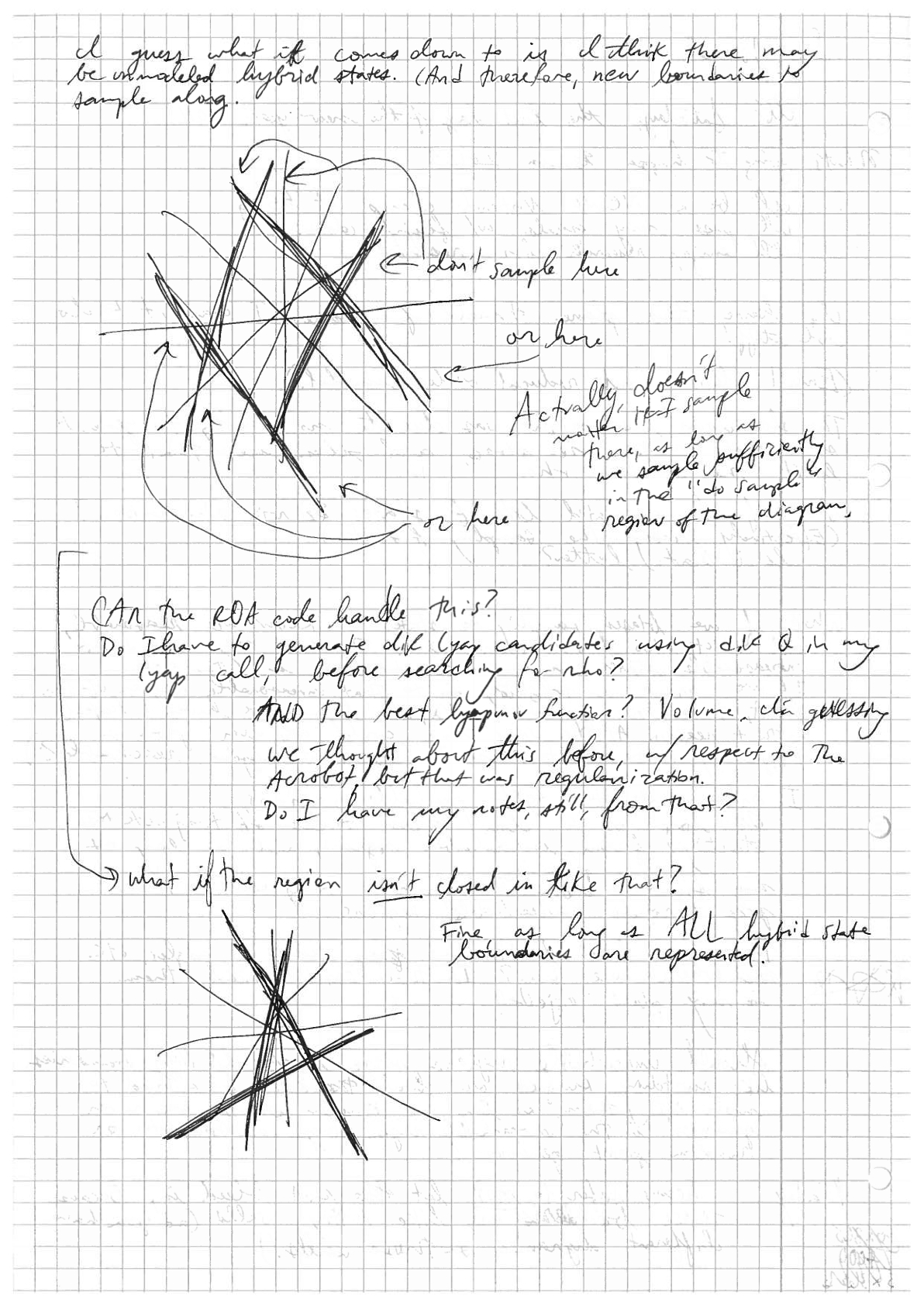
- notesfromRussphonemtg.pdf: Notes from today's phone meeting with Russ [in PDF form, reproduced below as an image]
- notesfromRussphonemtg.jpg:
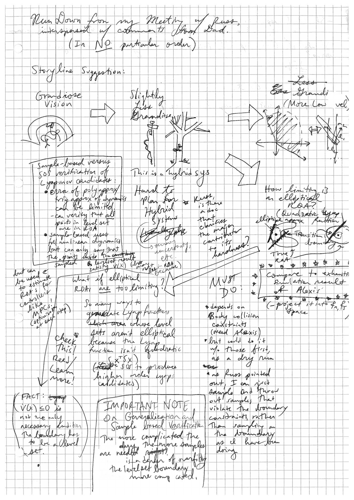
- The body-collisions that don't frequently (or ever) happen are still needed to restrict the size of the elliptical ROA approximation. (Therefore, we'll need them all!)
- Alexis' simpler model that he made over the break (airplane + leg with only one joint): has he had a chance to test it (simulate and visualize it) now that he doesn't have to use Matlab with a VPN? All I know about it is that it is the plane + leg with only one joint, but I wonder just how reduced a model that is. Rather than 8 states, we might still have 5 or so. What I remember us brainstorming before the break was a body with a leg. Essentially, a hip, no knee, no ankle. Two sticks, one representing the body, the other the leg, and the leg is attached somewhere in the middle of the body stick, with a torsional (?) spring at that (hip) joint. I think that's indeed what Alexis meant by plane + leg with only one joint. Awesome.
- Are body collisions checked for/accounted for in the simulator generated by Pauls software? Answer through email: The hybrid simulator only includes contact at the nose or tail with the wall, not the knee touching the wall, because it's rarely seen in practice and more complex. However, see first bullet point for why we still need it.
- What did Alexis mean by "Paul's software has no real "automated" way of doing this, but it is as simple as typing a single command line... so we can do this tomorrow" ?
- Talk to Alexis about how, even if, when following the natural dynamics of the system, one would almost always hit one transition boundary before another, we still need to consider both when determining the size of the ROA. (Very similar, if not the same, discussion as for first bullet point.)
- Add body collisions to AlexisPlane? plant object in robotlib
- Project ROA estimate into fn, fs space in order to see how conservative it is
- points called x lie in space A
- points called y lie in space B
- space A, B both have n dimensions, where n is the size of the state vector of the system we're working with
- space A is the actual state space of the system we're working with
Now we can generate a unit sphere of points in space B and map it to the ellipsoidal shell that is a particular level set of the lyapunov function in the state space. Very handy for our sample-based ROA approximation generation!
Also had a very productive meeting with Alexis today. We covered all the points I wrote down this morning (in the bulleted list above). Will bring this blog entry up to date with our decisions and the answers to my questions this evening.
First part of my update based on my discussion with Alexis:
We hammered out a plan. Turns out that we cannot know how conservative/appropriate the quadratic lyapunov candidates are for approximating the true ROA until Alexis runs a different script than the one that generated the landing envelope figures in his publications.
He does not have all the configuration constraints for the full model, and they're much simpler for the reduced order model, which he's currently testing to make sure it's correct.
Our plan is the following: - Tonight: He tests his reduced order model while I ready the code that can generate the sample-based ROA approximation, taking all hybrid state transition boundaries, including those defined by configuration constraints, into account. [I don't have the exact boundaries yet, but should tonight/tomorrow, as described below. But I'll make the code "ready to go" for when I have those exact conditions.]
- Tonight/tomorrow (whenever he's finished): he sends me the equations of motion of the reduced order model and the constraint equations (which are trivial but defined in terms of state variable definitions only he has)
- Tomorrow: I create a plant object for the reduced order model, plug it in to my code for generating sample-based ROAs, and project it into fn, fs space, while he runs a script (should take the script a couple hours to run on the Stanford cluster) to produce the analogous ROA by exhaustive simulation.
- Tomorrow/Thursday: we compare!
6Jan2010
This morning I woke up at sunrise and immediately finished debugging my code for using sampling to estimate the ROA. Alexis responded about a couple parameter values that would have to be the same in our respective pieces of code, and I made the appropriate parameter value changes to reflect his choices. While my code appears to be working properly, it's hard to know if there are any bugs still lurking in it because I have nothing to compare it to yet. Emailing Alexis about that now. I wonder if he's in the lab, and if his cluster has returned an ROA based on exhaustive simulation yet...
Thought a bit about how to only sample on the level set in the slice of state space defined by qH = 45 degrees, tailpenetration (or tailx?) = 0, since that's the slice Alexis is computing, but instead of a cute linear algebra solution, I tried some manipulation on the white board and decided it was easier and quicker to just sample in the space and mark with a color whether or not the point falls inside or outside the level set.
Accumulated To Do List - Check that I didn't make a silly mistake when computing value*DEGtoRAD or *RADtoDEG when hardcoding the values of the properties of the new hybrid model plants.
Classwork
- I have now watched lectures 1 - 14 of EE263, which is Prof. Boyd's class on linear dynamical systems.
- I now have access to the course materials of E (or EE?) 205.
- The meaning of zeros (not just poles) makes a lot more sense now, thanks to sitting in on some ME161 lectures.
- I am making my way quickly through MIT's 6.041 psets, to keep probabilistic system analysis fresh in my mind. I am having trouble with the "Prove this mathematical statement" type problems, though, especially those assigned in the graduate version of the class. I will have to keep revisiting that type of problem.
Ideas, requests, problems regarding TWiki? Send feedback