Prototype 3

The second prototype has confirmed the feasibility of copper mesh and temperature compensation sensor embedment in the 3-D exoskeletal robot finger structure. It has shown the ability of copper mesh to reduce the creep and thermal effect of a polymer based structure, as well as demonstrated that the isolated temperature compensation sensor has small dependency on external forces applied to the structure. However, in the implementation, only one FBG sensor was embedded in the skin structure that had limitation to localize or sense the applied force to the structure. The design goal of the third prototype was to remove this limitation. The effort focused on embedding multiple sensors and improving the inner structure for temperature compensation sensor embedment.

1. Design Modification and Improvement

The new prototype is shown in Figure 1. Four FBG sensors was embedded in the skin close to the joint at every 90 degrees and one temperature compensation sensor in the middle of the structure as shown in the figure. The temperature compensation sensor was placed inside a copper tube to minimize any possible strain changes caused by an external force application.

In addition, copper mesh was also embedded in the fingertip as well as in the skin to eliminate any unwanted deformation which could be another reason of creep effect of the structure. If the copper mesh was embedded only in the skin, the other part such as the fingertip or the joint would be relatively weaker.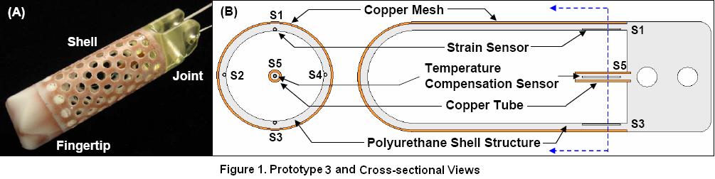

2. Material Selection

The same material (Task 3, Smooth-On, Easton, Pennsylvania, USA) was used for the skin and fingertip fabrication in the new prototype. However, harder and stiffer material (Task 9, Smooth-On, Easton, Pennsylvania, USA) was chosen for the joint fabrication to reduce the creep effect from the joint which did not have embedded copper mesh. Table 1 compares key properties of the two materials. The only drawback of Task 9 is its higher mixed viscosity than that of Task 3. However, it is not a big problem in the joint fabrication since the joint is not a thin shell type structure such as the fingertip or the skin, but a solid piece with a large top surface area of which all the air bubbles were removed. Figure 2 shows the clean bonding between two different materials.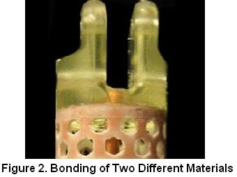

Table 1. Material Property Comparison

Material	Hardness	Flexural Modulus	Mixed Viscosity	Pot Life	Demold time
Task 3	80D	290 kpsi	150 cps	20 min	90 min
Task 9	85D	370 kpsi	300 cps	7 min	60 min

3. Finite Element Analysis

Although simple finite element analysis had already been carried out to find proper locations to embed FBG sensors using COSMOS Works® in the first quarter, more detailed FE analysis was needed to predict the behavior of the skin structure, so algorithms can be developed to localize the applied forces. Different forces on different locations of the skin structure were simulated, and the resultant strain changes at each sensor location recorded using ANSYS 8.1® in this stage.

3.1. Model Description and Conditions

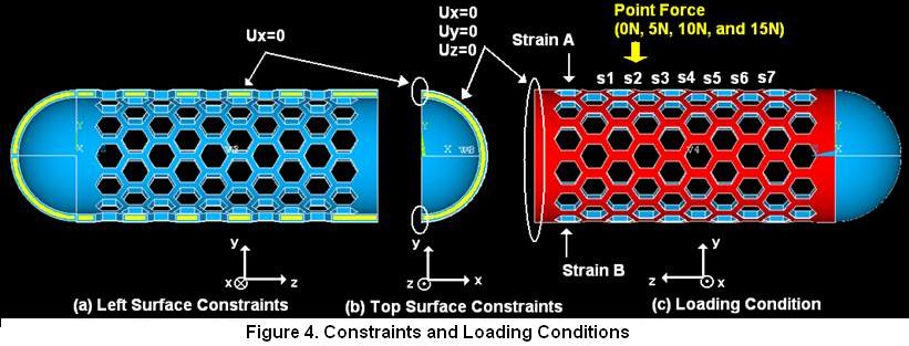
Figure 3 shows the half 3D ANSYS model of the prototype to be analyzed. Copper mesh was included in this model as shown in the figure, which was glued to the polyurethane skin structure, so the two different materials formed a combined layer that could move together. Figure 4 shows the constraints and loading conditions. The left surface of the half model is constrained only in x-axis as shown in Figure 4(a) due to the symmetry of the full model, and the top surface in all three axes as shown in Figure 4(b) since it will be attached to the fixed joint. As shown in Figure 4(c), point forces were applied to the different locations of the structure and strain changes at A and B in z-axis recorded.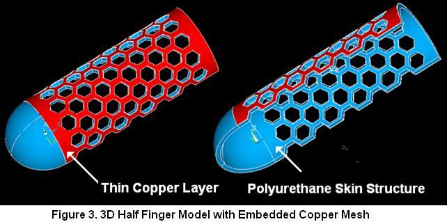

3.2 Analysis Results

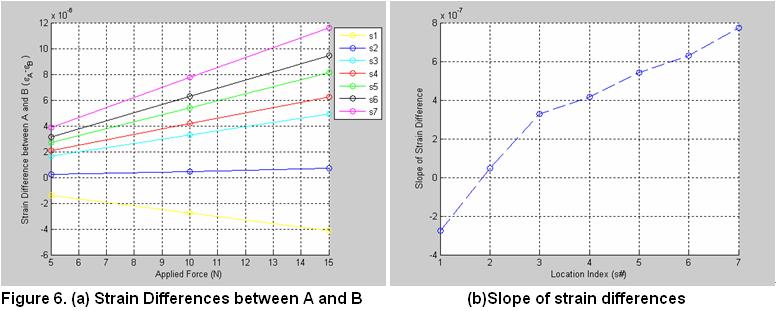
The main focus of this analysis is to develop simple algorithms to estimate the location of external force applications. There are two assumptions in this analysis; first, only a single force is applied at one time, and second, the direction of the applied forces is always normal to the surface.

3.2.1 Vertical Localization

Figure 5(a) shows strain changes at A and B for different forces on different spots as specified in Figure 4(c). Positive force means a force applied to the same side as the strain measurement and negative force the other side, so strain changes at A are plotted with positive forces and strain changes B with negative forces even though they result from the same force applications. Since the slope of strain changes at A and B are always consistent, we can simply calculate the ratio between the two strain changes as shown in Figure 5(b). As long as we know the exact ratio between the two strain changes, we can tell where the force is applied from the plot. However, since the strain ratio is not one to one mapping relative to the location, it is possible that the ratio from experiments is not exactly the same as from simulation. One way to solve this problem is to use dynamic force data. Figure 6(a) shows the differences of two strain changes from A and B, and their slopes are plotted in Figure 6(b). These slopes are always increasing as the force location becomes farther from the joint. Therefore, we can find vertical force locations as long as the system is fast enough to read the forces and their corresponding sensor outputs dynamically.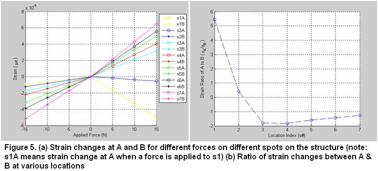

3.2.2 Horizontal Localization

It is not simple to find the force locations horizontally only with four sensor outputs. Figure 7 shows an example of one approach. If k is defined as:

k = (|Strain at A| - |Strain at B|) / ( |Strain at C| - |Strain at D| )

The system always has the same k value even though different forces are applied to the same spot.

If k = + infinite, force is on A, If k = – infinite, force is on B, If k = + zero, force is on C, and If k = – zero, force is on D.

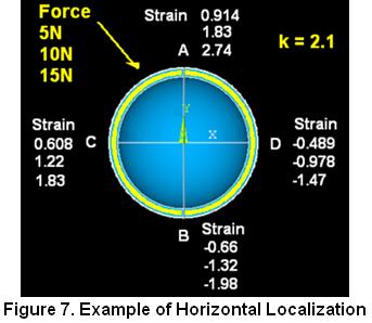This approach is not an exact method for horizontal localization since the k value may be different for different vertical locations. However, this shows the possibility of horizontal localization with only a few sensor outputs.

4. Force Sensing Test and Analysis

Since the I*SenseTM system was not calibrated to relate wavelength and strain during the tests, the sensor outputs shown in this report are all direct voltage output (V) from the interrogator system. However, the linearity of the output is the same as wavelength shift or strain changes basically.

4.1. Localization

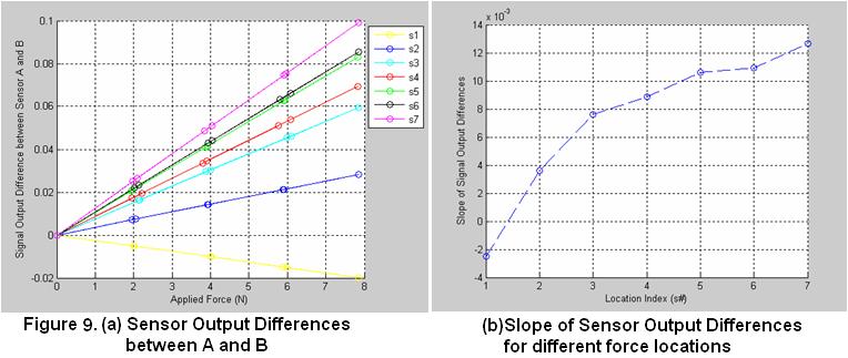
Vertical localization was attempted with the new prototype. Different forces were applied on various locations vertically in the manner described in the previous section, and their corresponding sensor outputs (A and B) were recorded. Figure 8(a) shows the sensor output for different forces, and its least-square fit is shown in Figure 8(b). Localization process was carried out using these least-square fits. The output signal ratio of sensor A to B is shown in Figure 8(c). One to one mapping is not shown in this figure. However, slopes of signal output differences make one to one mapping with force locations as shown in Figure 9(a). Compared to Figure 7(c), the tabulated results from the experiment, as shown in Figure 9(b), show the consistency with results obtained from finite element analysis.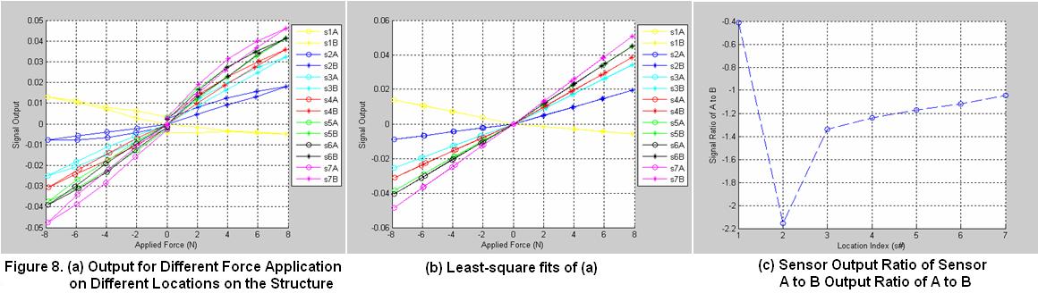

4.2. Dynamic Force Test

Dynamic force test has also been conducted as shown in Figure 10(a). A step input was given by removing a weight of 200g (1.962N) at a certain time. Sampling was made in every 100 s for 0.2 seconds. Settling time of much smaller than 0.1 seconds and approximately less than 2.5% overshoot are observed. Since the signal to noise ratio is 25.25 (= 0.0728 / 0.0004), the smallest force this system can measure is 0.0078N in static stage. Therefore, the system can measure a dynamic force larger than 0.0078N with faster than 10 Hz.

4.3. Thermal Effect Test

Figure 10(b) shows a dynamic thermal test result. Loading and unloading force was applied to the fingertip, and the temperature was decreased from 28.3C to 25.7C gradually during the test. Each number in the plot tells the temperature measured at each point. The result shows how fast and accurately temperature compensation sensor works.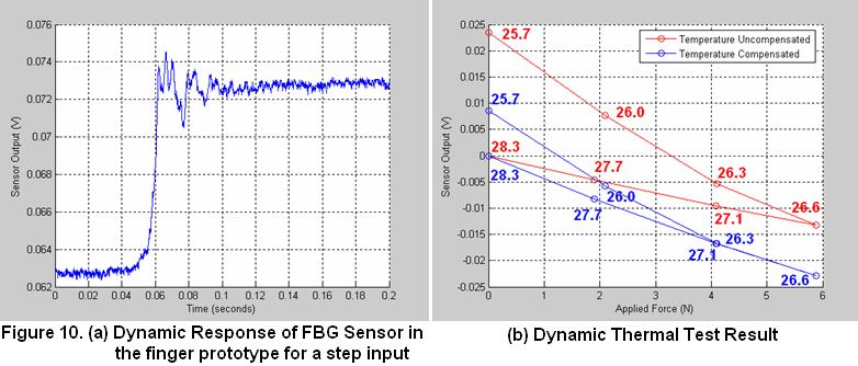

5. Conclusions and Future Work

Since the third prototype confirmed the feasibility of multiple FBG sensors for localization, more accurate localization algorithms will be developed using adaptive filtering. Then, the finger will be installed to the Stanford Dexter robot arm for closed loop feedback control. We will continue to refine our fabrication processes and improve our yield, especially developing a technique to reduce stress on fibers due to embedment process. We plan to have one more run on the current design with few enhancements, i.e. optical losses, fiber management and interface to Stanford Dexter robot arm.

-- YongLaePark - 20 Sep 2006